---
license: cc-by-sa-4.0
metrics:
- mse
pipeline_tag: graph-ml
---
# AIFS Single - v0.2.1
Here, we introduce the **Artificial Intelligence Forecasting System (AIFS)**, a data driven forecast
model developed by the European Centre for Medium-Range Weather Forecasts (ECMWF).
We show that AIFS produces highly skilled forecasts for upper-air variables, surface weather parameters and
tropical cyclone tracks. AIFS is run four times daily alongside ECMWF’s physics-based NWP model and forecasts
are available to the public under ECMWF’s open data policy. (https://www.ecmwf.int/en/forecasts/datasets/open-data)
## Model Details
### Model Description
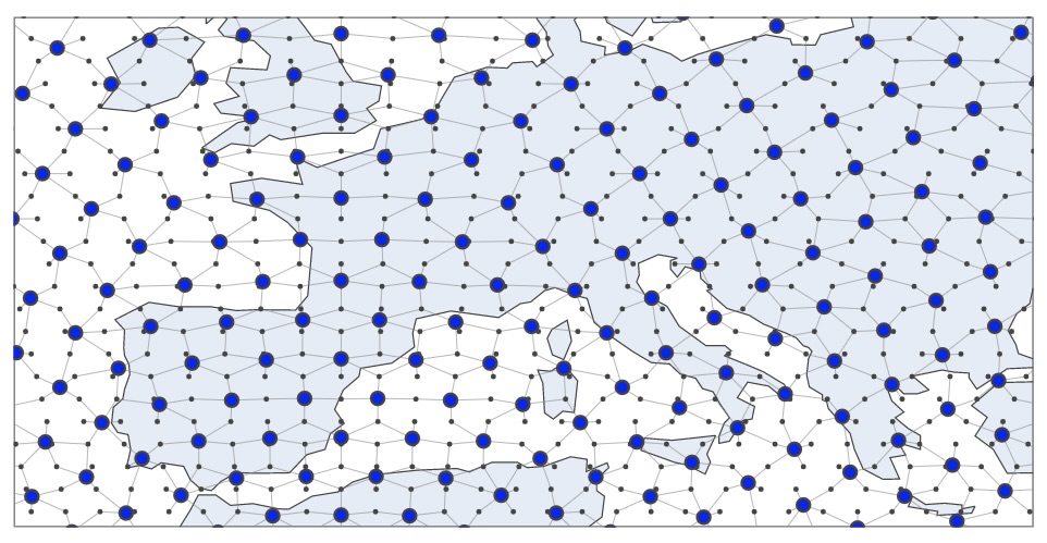
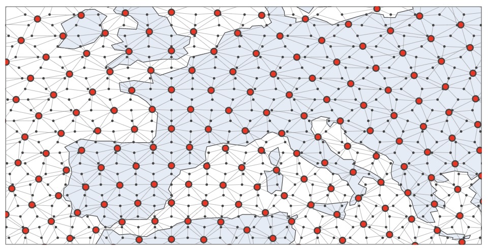
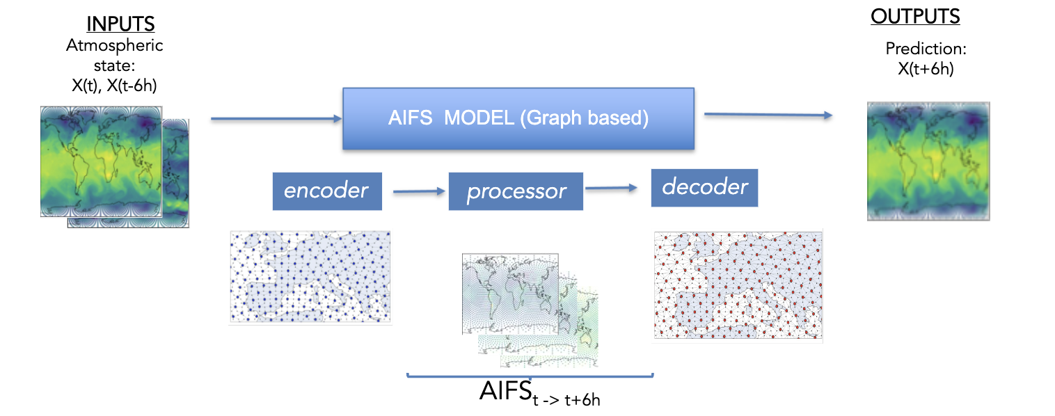
AIFS is based on a graph neural network (GNN) encoder and decoder, and a sliding window transformer processor,
and is trained on ECMWF’s ERA5 re-analysis and ECMWF’s operational numerical weather prediction (NWP) analyses.
It has a flexible and modular design and supports several levels of parallelism to enable training on
high resolution input data. AIFS forecast skill is assessed by comparing its forecasts to NWP analyses
and direct observational data.
- **Developed by:** ECMWF
- **Model type:** Encoder-processor-decoder model
- **License:** CC BY-SA 4.0
### Model Sources
- **Repository:** [Anemoi](https://anemoi-docs.readthedocs.io/en/latest/index.html)
Anemoi is an open-source framework for creating machine learning (ML) weather forecasting systems, which ECMWF and a range of national meteorological services across Europe have co-developed.
- **Paper:** https://arxiv.org/pdf/2406.01465
## How to Get Started with the Model
To be able to run AIFS to generate a new forecast, you can use ai-models https://github.com/ecmwf-lab/ai-models.
`ai-models` command can be used to run different models, since in this case we are looking at using AIFS we need to specify
`anemoi` as `model-name` and then pass the path to the checkpoint (`aifs_single_v0.2.1.ckpt`) and the initial conditions.
You can find an example of a set of initial conditions in the GRIB file `example_20241107_12_n320.grib`.
Use the code below to get started with the model.
```
# 1st - create the conda environment
export CONDA_ENV=aifs-env
conda create -n ${CONDA_ENV} python=3.10
conda activate ${CONDA_ENV}
pip install torch=2.4
pip install anemoi-inference[plugin] anemoi-models==0.2
pip install ninja
pip install flash-attn --no-build-isolation
# 2nd - Run ai-models to generate weather forecast
ai-models anemoi --checkpoint aifs_single_v0.2.1.ckpt --file example_20241107_12_n320.grib
```
🚨 **Note** we train AIFS using `flash_attention` (https://github.com/Dao-AILab/flash-attention).
There are currently some issues when trying to install flash attention with the latest PyTorch version 2.5 and CUDA 12.4 (https://github.com/Dao-AILab/flash-attention/issues/1330).
For that reason, we recommend you install PyTorch 2.4.
Additonally the use of 'Flash Attention' package also imposes certain requirements in terms of software and hardware. Those can be found under #Installation and Features in https://github.com/Dao-AILab/flash-attention
🚨 **Note** the `aifs_single_v0.2.1.ckpt` checkpoint just contains the model’s weights.
That file does not contain any information about the optimizer states, lr-scheduler states, etc.
**Note** By default, when running `ai-models` the model will be run for a 10-day lead time (240 hours).
It is possible to extend or modify the lead time to for example 15 days by doing `ai-models --lead-time 360`
Please refer to `ai-models` documentation for more information regarding defaults and available command line options.
After running the `ai-models` command the output of the forecast should be written into `anemoi.grib`
Below you can find an example to read that file and load it as numpy array or xarray.
```
import earthkit.data as ekd
source_filename='anemoi.grib'
aifs_forecast = ekd.from_source('file',source_filename)
# to load it as a numpy array
aifs_forecast.to_numpy() #
# to load it as a xarray array
aifs_forecast.to_xarray()
```
## Training Details
### Training Data
AIFS is trained to produce 6-hour forecasts. It receives as input a representation of the atmospheric states
at \\(t_{−6h}\\), \\(t_{0}\\), and then forecasts the state at time \\(t_{+6h}\\).
The full list of input and output fields is shown below:
| Field | Level type | Input/Output |
|-------------------------------------------------------------------------------------------------------------------------------------------------------------|------------------------------------------------------------------------------|--------------|
| Geopotential, horizontal and vertical wind components, specific humidity, temperature | Pressure level: 50,100, 150, 200, 250,300, 400, 500, 600,700, 850, 925, 1000 | Both |
| Surface pressure, mean sea-level pressure, skin temperature, 2 m temperature, 2 m dewpoint temperature, 10 m horizontal wind components, total column water | Surface | Both |
| Total precipitation, convective precipitation | Surface | Output |
| Land-sea mask, orography, standard deviation of sub-grid orography, slope of sub-scale orography, insolation, latitude/longitude, time of day/day of year | Surface | Input |
Input and output states are normalised to unit variance and zero mean for each level. Some of
the forcing variables, like orography, are min-max normalised.
### Training Procedure
- **Pre-training**: It was performed on ERA5 for the years 1979 to 2020 with a cosine learning rate (LR) schedule and a total
of 260,000 steps. The LR is increased from 0 to \\(10^{-4}\\) during the first 1000 steps, then it is annealed to a minimum
of \\(3 × 10^{-7}\\).
- **Fine-tuning I**: The pre-training is then followed by rollout on ERA5 for the years 1979 to 2018, this time with a LR
of \\(6 × 10^{-7}\\). As in [Lam et al. [2023]](doi: 10.21957/slk503fs2i) we increase the
rollout every 1000 training steps up to a maximum of 72 h (12 auto-regressive steps).
- **Fine-tuning II**: Finally, to further improve forecast performance, we fine-tune the model on operational real-time IFS NWP
analyses. This is done via another round of rollout training, this time using IFS operational analysis data
from 2019 and 2020
#### Training Hyperparameters
- **Optimizer:** We use *AdamW* (Loshchilov and Hutter [2019]) with the \\(β\\)-coefficients set to 0.9 and 0.95.
- **Loss function:** The loss function is an area-weighted mean squared error (MSE) between the target atmospheric state
and prediction.
- **Loss scaling:** A loss scaling is applied for each output variable. The scaling was chosen empirically such that
all prognostic variables have roughly equal contributions to the loss, with the exception of the vertical velocities,
for which the weight was reduced. The loss weights also decrease linearly with height, which means that levels in
the upper atmosphere (e.g., 50 hPa) contribute relatively little to the total loss value.
#### Speeds, Sizes, Times
Data parallelism is used for training, with a batch size of 16. One model instance is split across four 40GB A100
GPUs within one node. Training is done using mixed precision (Micikevicius et al. [2018]), and the entire process
takes about one week, with 64 GPUs in total. The checkpoint size is 1.19 GB and it does not include the optimizer
state.
## Evaluation
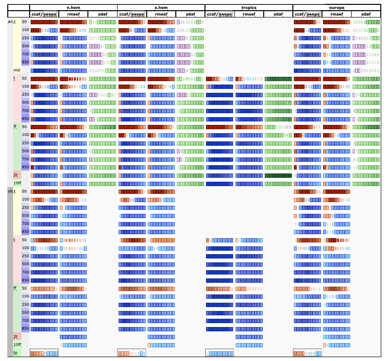
AIFS is evaluated against ECMWF IFS (Integrated Forecast System) for 2022. The results of such evaluation are summarized in
the scorecard below that compares different forecast skill measures across a range of
variables. For verification, each system is compared against the operational ECMWF analysis from which the forecasts
are initialised. In addition, the forecasts are compared against radiosonde observations of geopotential, temperature
and windspeed, and SYNOP observations of 2 m temperature, 10 m wind and 24 h total precipitation. The definition
of the metrics, such as ACC (ccaf), RMSE (rmsef) and forecast activity (standard deviation of forecast anomaly,
sdaf) can be found in e.g Ben Bouallegue et al. ` [2024].
Forecasts are initialised on 00 and 12 UTC. The scorecard show relative score changes as function of lead time (day 1 to 10) for northern extra-tropics (n.hem),
southern extra-tropics (s.hem), tropics and Europe. Blue colours mark score improvements and red colours score
degradations. Purple colours indicate an increased in standard deviation of forecast anomaly, while green colours
indicate a reduction. Framed rectangles indicate 95% significance level. Variables are geopotential (z), temperature
(t), wind speed (ff), mean sea level pressure (msl), 2 m temperature (2t), 10 m wind speed (10ff) and 24 hr total
precipitation (tp). Numbers behind variable abbreviations indicate variables on pressure levels (e.g., 500 hPa), and
suffix indicates verification against IFS NWP analyses (an) or radiosonde and SYNOP observations (ob). Scores
shown are anomaly correlation (ccaf), SEEPS (seeps, for precipitation), RMSE (rmsef) and standard deviation of
forecast anomaly (sdaf, see text for more explanation).
Additional evaluation analysis including tropycal cyclone performance or comparison against other popular data-driven models can be found in AIFS preprint (https://arxiv.org/pdf/2406.01465v1) section 4.
# Known limitations
- This version of AIFS shares certain limitations with some of the other data-driven weather forecast models that are trained with a weighted MSE loss, such as blurring of the forecast fields at longer lead times.
- AIFS exhibits reduced forecast skill in the stratosphere forecast owing to the linear loss scaling with height
- AIFS currently provides reduced intensity of some high-impact systems such as tropical cyclones.
## Technical Specifications
### Hardware
We acknowledge PRACE for awarding us access to Leonardo, CINECA, Italy. In particular, this version of the AIFS has been trained
on 64 A100 GPUs (40GB).
### Software
The model was developed and trained using the [AnemoI framework](https://anemoi-docs.readthedocs.io/en/latest/index.html).
AnemoI is a framework for developing machine learning weather forecasting models. It comprises of components or packages
for preparing training datasets, conducting ML model training and a registry for datasets and trained models. AnemoI
provides tools for operational inference, including interfacing to verification software. As a framework it seeks to
handle many of the complexities that meteorological organisations will share, allowing them to easily train models from
existing recipes but with their own data.
## Citation
If you use this model in your work, please cite it as follows:
**BibTeX:**
```
@article{lang2024aifs,
title={AIFS-ECMWF's data-driven forecasting system},
author={Lang, Simon and Alexe, Mihai and Chantry, Matthew and Dramsch, Jesper and Pinault, Florian and Raoult, Baudouin and Clare, Mariana CA and Lessig, Christian and Maier-Gerber, Michael and Magnusson, Linus and others},
journal={arXiv preprint arXiv:2406.01465},
year={2024}
}
```
**APA:**
```
Lang, S., Alexe, M., Chantry, M., Dramsch, J., Pinault, F., Raoult, B., ... & Rabier, F. (2024). AIFS-ECMWF's data-driven forecasting system. arXiv preprint arXiv:2406.01465.
```
## More Information
[More Information Needed](https://arxiv.org/pdf/2406.01465)


