# Working with Streaming Data
"Streaming data" is data that is continuously generated, often by some external source like a remote website, a measuring device, or a simulator. This kind of data is common for financial time series, web server logs, scientific applications, and many other situations. We have seen how to visualize any data output by a callable in the [Live Data](07-Live_Data.ipynb) user guide and we have also seen how to use the HoloViews stream system to push events in the user guide sections [Responding to Events](12-Responding_to_Events.ipynb) and [Custom Interactivity](13-Custom_Interactivity.ipynb).
This user guide shows a third way of building an interactive plot, using ``DynamicMap`` and streams. Here, instead of pushing plot metadata (such as zoom ranges, user triggered events such as ``Tap`` and so on) to a ``DynamicMap`` callback, the underlying data in the visualized elements are updated directly using a HoloViews ``Stream``.
In particular, we will show how the HoloViews ``Pipe`` and ``Buffer`` streams can be used to work with streaming data sources without having to fetch or generate the data from inside the ``DynamicMap`` callable. Apart from simply setting element data from outside a ``DynamicMap``, we will also explore ways of working with streaming data coordinated by the separate [``streamz``](http://matthewrocklin.com/blog/work/2017/10/16/streaming-dataframes-1) library from Matt Rocklin, which can make building complex streaming pipelines much simpler.
As this notebook makes use of the ``streamz`` library, you will need to install it with ``conda install streamz`` or ``pip install streamz``.
```python
import time
import numpy as np
import pandas as pd
import holoviews as hv
import streamz
import streamz.dataframe
from holoviews import opts
from holoviews.streams import Pipe, Buffer
hv.extension('bokeh')
```
## ``Pipe``
A ``Pipe`` allows data to be pushed into a DynamicMap callback to change a visualization, just like the streams in the [Responding to Events](./12-Responding_to_Events.ipynb) user guide were used to push changes to metadata that controlled the visualization. A ``Pipe`` can be used to push data of any type and make it available to a ``DynamicMap`` callback. Since all ``Element`` types accept ``data`` of various forms we can use ``Pipe`` to push data directly to the constructor of an ``Element`` through a DynamicMap.
We can take advantage of the fact that most Elements can be instantiated without providing any data, so we declare the the ``Pipe`` with an empty list, declare the ``DynamicMap``, providing the pipe as a stream, which will dynamically update a ``VectorField`` :
```python
pipe = Pipe(data=[])
vector_dmap = hv.DynamicMap(hv.VectorField, streams=[pipe])
vector_dmap.opts(color='Magnitude', xlim=(-1, 1), ylim=(-1, 1))
```
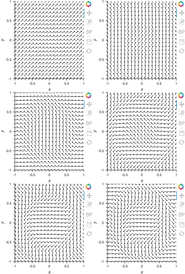 Having set up this ``VectorField`` tied to a ``Pipe`` we can start pushing data to it varying the orientation of the VectorField:
```python
x,y = np.mgrid[-10:11,-10:11] * 0.1
sine_rings = np.sin(x**2+y**2)*np.pi+np.pi
exp_falloff = 1/np.exp((x**2+y**2)/8)
for i in np.linspace(0, 1, 25):
time.sleep(0.1)
pipe.send((x,y,sine_rings*i, exp_falloff))
```
This approach of using an element constructor directly does not allow you to use anything other than the default key and value dimensions. One simple workaround for this limitation is to use ``functools.partial`` as demonstrated in the **Controlling the length section** below.
Since ``Pipe`` is completely general and the data can be any custom type, it provides a completely general mechanism to stream structured or unstructured data. Due to this generality, ``Pipe`` does not offer some of the more complex features and optimizations available when using the ``Buffer`` stream described in the next section.
## ``Buffer``
While ``Pipe`` provides a general solution for piping arbitrary data to ``DynamicMap`` callback, ``Buffer`` on the other hand provides a very powerful means of working with streaming tabular data, defined as pandas dataframes, arrays or dictionaries of columns (as well as StreamingDataFrame, which we will cover later). ``Buffer`` automatically accumulates the last ``N`` rows of the tabular data, where ``N`` is defined by the ``length``.
The ability to accumulate data allows performing operations on a recent history of data, while plotting backends (such as bokeh) can optimize plot updates by sending just the latest patch. This optimization works only if the ``data`` object held by the ``Buffer`` is identical to the plotted ``Element`` data, otherwise all the data will be updated as normal.
#### A simple example: Brownian motion
To initialize a ``Buffer`` we have to provide an example dataset which defines the columns and dtypes of the data we will be streaming. Next we define the ``length`` to keep the last 100 rows of data. If the data is a DataFrame we can specify whether we will also want to use the ``DataFrame`` ``index``. In this case we will simply define that we want to plot a ``DataFrame`` of 'x' and 'y' positions and a 'count' as ``Points`` and ``Curve`` elements:
```python
example = pd.DataFrame({'x': [], 'y': [], 'count': []}, columns=['x', 'y', 'count'])
dfstream = Buffer(example, length=100, index=False)
curve_dmap = hv.DynamicMap(hv.Curve, streams=[dfstream])
point_dmap = hv.DynamicMap(hv.Points, streams=[dfstream])
```
After applying some styling we will display an ``Overlay`` of the dynamic ``Curve`` and ``Points``
```python
(curve_dmap * point_dmap).opts(
opts.Points(color='count', line_color='black', size=5, padding=0.1, xaxis=None, yaxis=None),
opts.Curve(line_width=1, color='black'))
```
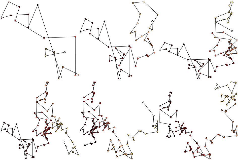 Now that we have set up the ``Buffer`` and defined a ``DynamicMap`` to plot the data we can start pushing data to it. We will define a simple function which simulates brownian motion by accumulating x, y positions. We can ``send`` data through the ``hv.streams.Buffer`` directly.
```python
def gen_brownian():
x, y, count = 0, 0, 0
while True:
x += np.random.randn()
y += np.random.randn()
count += 1
yield pd.DataFrame([(x, y, count)], columns=['x', 'y', 'count'])
brownian = gen_brownian()
for i in range(200):
dfstream.send(next(brownian))
```
Finally we can clear the data on the stream and plot using the ``clear`` method:
```python
dfstream.clear()
```
Note that when using the ``Buffer`` stream the view will always follow the current range of the data by default, by setting ``buffer.following=False`` or passing following as an argument to the constructor this behavior may be disabled.
## Using the Streamz library
Now that we have discovered what ``Pipe`` and ``Buffer`` can do it's time to show how you can use them together with the ``streamz`` library. Although HoloViews does not depend on ``streamz`` and you can use the streaming functionality without needing to learn about it, the two libraries work well together, allowing you to build pipelines to manage continuous streams of data. Streamz is easy to use for simple tasks, but also supports complex pipelines that involve branching, joining, flow control, feedback and more. Here we will mostly focus on connecting streamz output to ``Pipe`` and then ``Buffer`` so for more details about the streamz API, consult the [streamz documentation](https://streamz.readthedocs.io/en/latest/).
#### Using ``streamz.Stream`` together with ``Pipe``
Let's start with a fairly simple example:
1. Declare a ``streamz.Stream`` and a ``Pipe`` object and connect them into a pipeline into which we can push data.
2. Use a ``sliding_window`` of 10, which will first wait for 10 sets of stream updates to accumulate. At that point and for every subsequent update, it will apply ``pd.concat`` to combine the most recent 10 updates into a new dataframe.
3. Use the ``sink`` method on the ``streamz.Stream`` to ``send`` the resulting collection of 10 updates to ``Pipe``.
4. Declare a ``DynamicMap`` that takes the sliding window of concatenated DataFrames and displays it using a ``Scatter`` Element.
5. Color the ``Scatter`` points by their 'count' and set a range, then display:
```python
point_source = streamz.Stream()
pipe = Pipe(data=pd.DataFrame({'x': [], 'y': [], 'count': []}))
point_source.sliding_window(20).map(pd.concat).sink(pipe.send) # Connect streamz to the Pipe
scatter_dmap = hv.DynamicMap(hv.Scatter, streams=[pipe])
```
After set up our streaming pipeline we can again display it:
```python
scatter_dmap.opts(bgcolor='black', color='count', ylim=(-4, 4), show_legend=False)
```
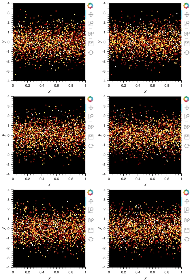 There is now a pipeline, but initially this plot will be empty, because no data has been sent to it. To see the plot update, let's use the ``emit`` method of ``streamz.Stream`` to send small chunks of random pandas ``DataFrame``s to our plot:
```python
for i in range(100):
df = pd.DataFrame({'x': np.random.rand(100), 'y': np.random.randn(100), 'count': i},
columns=['x', 'y', 'count'])
point_source.emit(df)
```
#### Using StreamingDataFrame and StreamingSeries
The streamz library provides ``StreamingDataFrame`` and ``StreamingSeries`` as a powerful way to easily work with live sources of tabular data. This makes it perfectly suited to work with ``Buffer``. With the ``StreamingDataFrame`` we can easily stream data, apply computations such as cumulative and rolling statistics and then visualize the data with HoloViews.
The ``streamz.dataframe`` module provides a ``Random`` utility that generates a ``StreamingDataFrame`` that emits random data with a certain frequency at a specified interval. The ``example`` attribute lets us see the structure and dtypes of the data we can expect:
```python
simple_sdf = streamz.dataframe.Random(freq='10ms', interval='100ms')
print(simple_sdf.index)
simple_sdf.example.dtypes
```
Since the ``StreamingDataFrame`` provides a pandas-like API, we can specify operations on the data directly. In this example we subtract a fixed offset and then compute the cumulative sum, giving us a randomly drifting timeseries. We can then pass the x-values of this dataframe to the HoloViews ``Buffer`` and supply ``hv.Curve`` as the ``DynamicMap`` callback to stream the data into a HoloViews ``Curve`` (with the default key and value dimensions):
```python
sdf = (simple_sdf-0.5).cumsum()
hv.DynamicMap(hv.Curve, streams=[Buffer(sdf.x)]).opts(width=500, show_grid=True)
```
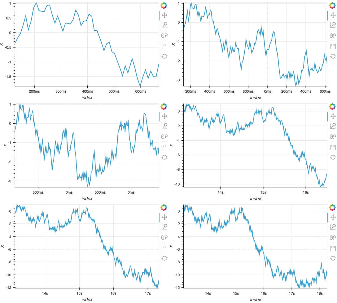 The ``Random`` StreamingDataFrame will asynchronously emit events, driving the visualization forward, until it is explicitly stopped, which we can do by calling the ``stop`` method.
```python
simple_sdf.stop()
```
#### Making use of the ``StreamingDataFrame`` API
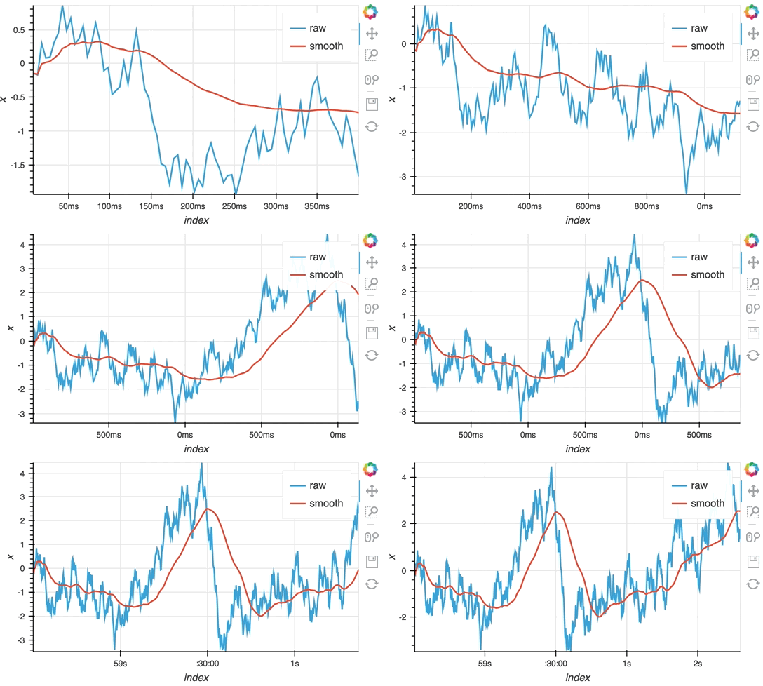
So far we have only computed the cumulative sum, but the ``StreamingDataFrame`` actually has an extensive API that lets us run a broad range of streaming computations on our data. For example, let's apply a rolling mean to our x-values with a window of 500ms and overlay it on top of the 'raw' data:
```python
source_df = streamz.dataframe.Random(freq='5ms', interval='100ms')
sdf = (source_df-0.5).cumsum()
raw_dmap = hv.DynamicMap(hv.Curve, streams=[Buffer(sdf.x)])
smooth_dmap = hv.DynamicMap(hv.Curve, streams=[Buffer(sdf.x.rolling('500ms').mean())])
(raw_dmap.relabel('raw') * smooth_dmap.relabel('smooth')).opts(
opts.Curve(width=500, show_grid=True))
```
 ```python
source_df.stop()
```
#### Customizing elements with ``functools.partial``
In this notebook we have avoided defining custom functions for ``DynamicMap`` by simply supplying the element class and using the element constructor instead. Although this works well for examples, it often won't generalize to real-life situations, because you don't have an opportunity to use anything other than the default dimensions. One simple way to get around this limitation is to use ``functools.partial``:
```python
from functools import partial
```
Now you can now easily create an inline callable that creates an element with custom key and value dimensions by supplying them to ``partial`` in the form ``partial(hv.Element, kdims=[...], vdims=[...])``. In the next section, we will see an example of this pattern using ``hv.BoxWhisker``.
#### Controlling the length
By default the ``Buffer`` accumulates a ``length`` of 1000 samples. In many cases this may be excessive, but we can specify a shorter (or longer) length value to control how much history we accumulate, often depending on the element type.
In the following example, a custom ``length`` is used together with a ``partial`` wrapping ``hv.BoxWhisker`` in order to display a cumulative sum generated from a stream of random dataframes:
```python
multi_source = streamz.dataframe.Random(freq='50ms', interval='500ms')
sdf = (multi_source-0.5).cumsum()
hv.DynamicMap(hv.Table, streams=[Buffer(sdf.x, length=10)]) +\
hv.DynamicMap(partial(hv.BoxWhisker, kdims=[], vdims='x'), streams=[Buffer(sdf.x, length=100)])
```
```python
source_df.stop()
```
#### Customizing elements with ``functools.partial``
In this notebook we have avoided defining custom functions for ``DynamicMap`` by simply supplying the element class and using the element constructor instead. Although this works well for examples, it often won't generalize to real-life situations, because you don't have an opportunity to use anything other than the default dimensions. One simple way to get around this limitation is to use ``functools.partial``:
```python
from functools import partial
```
Now you can now easily create an inline callable that creates an element with custom key and value dimensions by supplying them to ``partial`` in the form ``partial(hv.Element, kdims=[...], vdims=[...])``. In the next section, we will see an example of this pattern using ``hv.BoxWhisker``.
#### Controlling the length
By default the ``Buffer`` accumulates a ``length`` of 1000 samples. In many cases this may be excessive, but we can specify a shorter (or longer) length value to control how much history we accumulate, often depending on the element type.
In the following example, a custom ``length`` is used together with a ``partial`` wrapping ``hv.BoxWhisker`` in order to display a cumulative sum generated from a stream of random dataframes:
```python
multi_source = streamz.dataframe.Random(freq='50ms', interval='500ms')
sdf = (multi_source-0.5).cumsum()
hv.DynamicMap(hv.Table, streams=[Buffer(sdf.x, length=10)]) +\
hv.DynamicMap(partial(hv.BoxWhisker, kdims=[], vdims='x'), streams=[Buffer(sdf.x, length=100)])
```
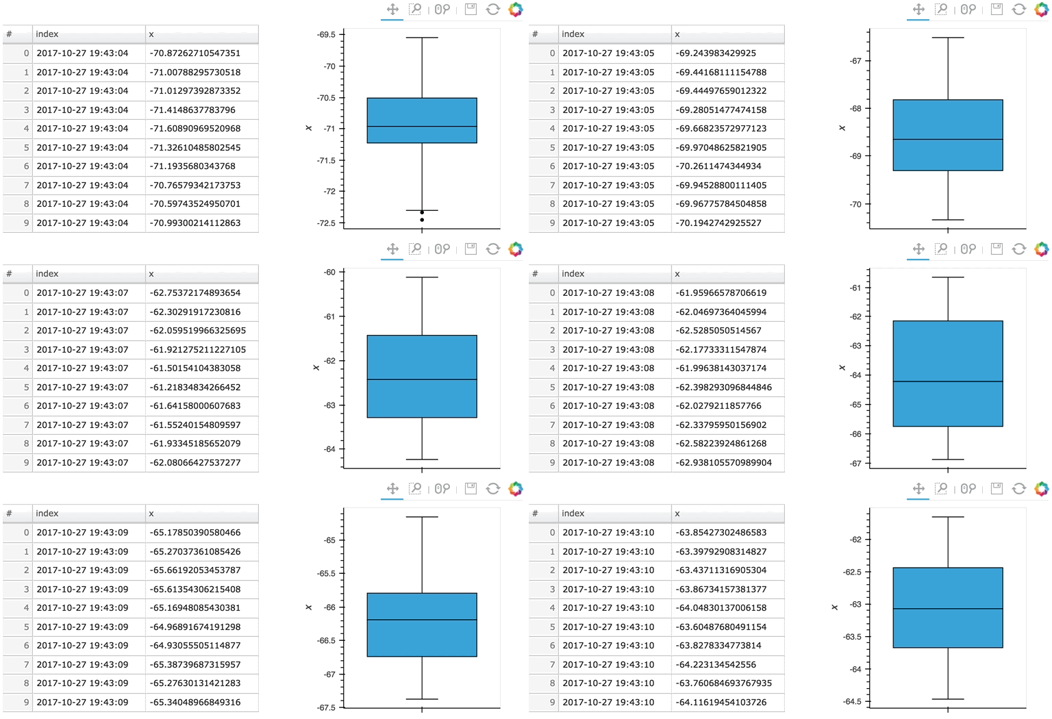 Here the given stream ``sdf`` is being consumed by a table showing a short length (where only the items visible in the table need to be kept), along with a plot computing averages and variances over a longer length (100 items).
#### Updating multiple cells
Since a ``StreamingDataFrame`` will emit data until it is stopped, we can subscribe multiple plots across different cells to the same stream. Here, let's add a ``Scatter`` plot of the same data stream as in the preceding cell:
```python
hv.DynamicMap(hv.Scatter, streams=[Buffer(sdf.x)]).redim.label(x='value', index='time')
```
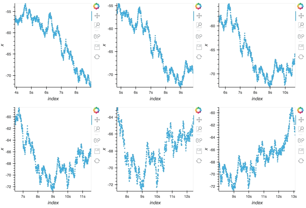 Here we let the ``Scatter`` elements use the column names from the supplied ``DataFrames`` which are relabelled using the ``redim`` method. Stopping the stream will now stop updates to all three of these DynamicMaps:
```python
multi_source.stop()
```
## Operations over streaming data
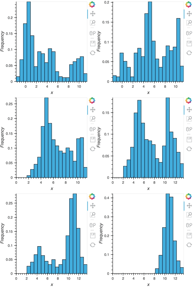
As we discovered above, the ``Buffer`` lets us set a ``length``, which defines how many rows we want to accumulate. We can use this to our advantage and apply an operation over this length window. In this example we declare a ``Dataset`` and then apply the ``histogram`` operation to compute a ``Histogram`` over the specified ``length`` window:
```python
hist_source = streamz.dataframe.Random(freq='5ms', interval='100ms')
sdf = (hist_source-0.5).cumsum()
dmap = hv.DynamicMap(hv.Dataset, streams=[Buffer(sdf.x, length=500)])
hv.operation.histogram(dmap, dimension='x')
```
 ```python
hist_source.stop()
```
#### Datashading
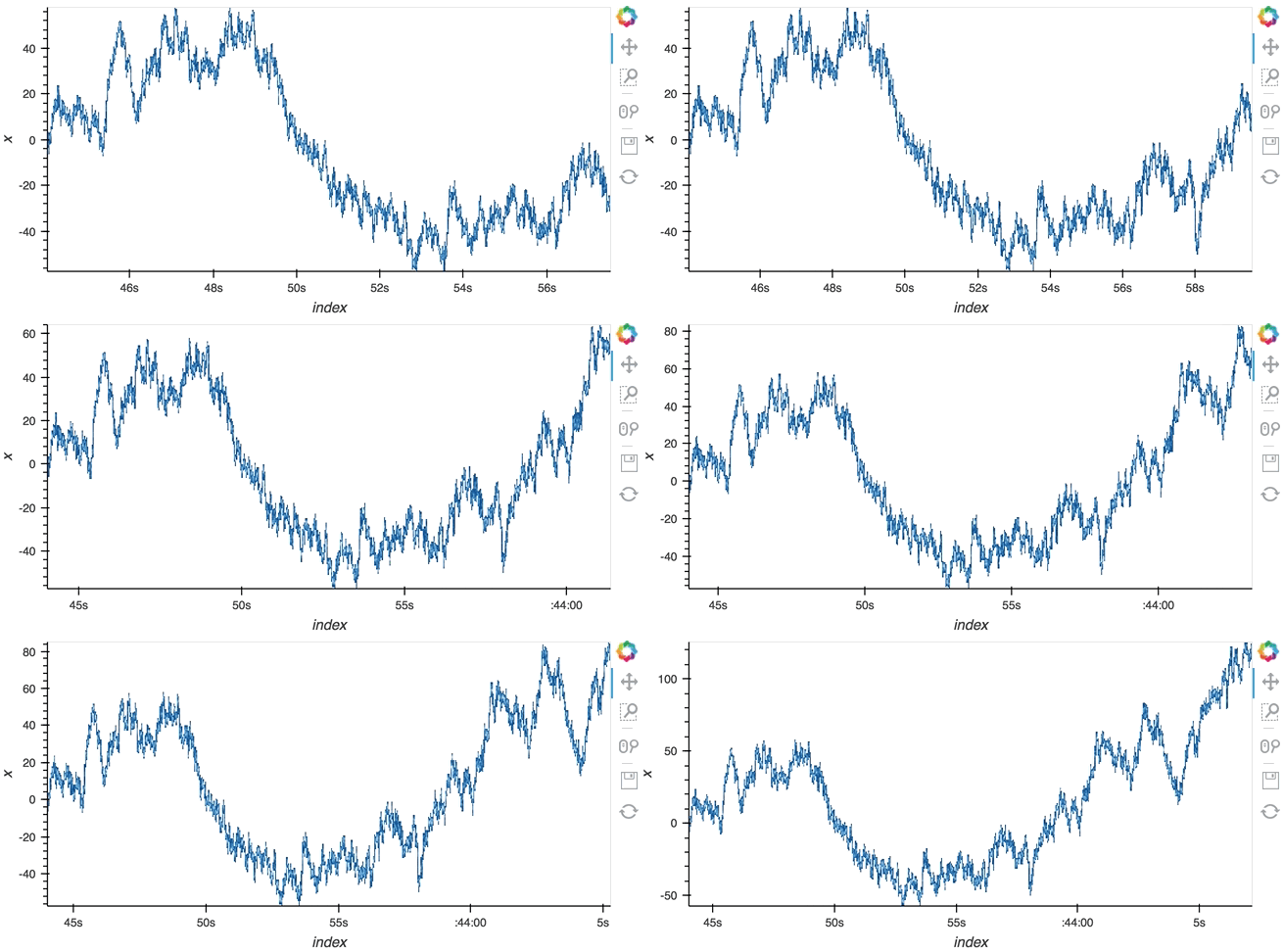
The same approach will also work for the datashader operation letting us datashade the entire ``length`` window even if we make it very large such as 1 million samples:
```python
from holoviews.operation.datashader import datashade
from bokeh.palettes import Blues8
large_source = streamz.dataframe.Random(freq='100us', interval='200ms')
sdf = (large_source-0.5).cumsum()
dmap = hv.DynamicMap(hv.Curve, streams=[Buffer(sdf.x, length=1000000)])
datashade(dmap, streams=[hv.streams.PlotSize], cnorm='linear', cmap=list(Blues8)).opts(width=600)
```
```python
hist_source.stop()
```
#### Datashading
The same approach will also work for the datashader operation letting us datashade the entire ``length`` window even if we make it very large such as 1 million samples:
```python
from holoviews.operation.datashader import datashade
from bokeh.palettes import Blues8
large_source = streamz.dataframe.Random(freq='100us', interval='200ms')
sdf = (large_source-0.5).cumsum()
dmap = hv.DynamicMap(hv.Curve, streams=[Buffer(sdf.x, length=1000000)])
datashade(dmap, streams=[hv.streams.PlotSize], cnorm='linear', cmap=list(Blues8)).opts(width=600)
```
 ```python
large_source.stop()
```
## Asynchronous updates using the tornado ``IOLoop``
In most cases, instead of pushing updates manually from the same Python process, you'll want the object to update asynchronously as new data arrives. Since both Jupyter and Bokeh server run on [tornado](http://www.tornadoweb.org/en/stable/), we can use the tornado ``IOLoop`` in both cases to define a non-blocking co-routine that can push data to our stream whenever it is ready. The ``PeriodicCallback`` makes this approach very simple, we simply define a function which will be called periodically with a timeout defined in milliseconds. Once we have declared the callback we can call ``start`` to begin emitting events:
```python
from tornado.ioloop import PeriodicCallback
from tornado import gen
count = 0
buffer = Buffer(np.zeros((0, 2)), length=50)
@gen.coroutine
def f():
global count
count += 1
buffer.send(np.array([[count, np.random.rand()]]))
cb = PeriodicCallback(f, 100)
cb.start()
hv.DynamicMap(hv.Curve, streams=[buffer]).opts(padding=0.1, width=600)
```
```python
large_source.stop()
```
## Asynchronous updates using the tornado ``IOLoop``
In most cases, instead of pushing updates manually from the same Python process, you'll want the object to update asynchronously as new data arrives. Since both Jupyter and Bokeh server run on [tornado](http://www.tornadoweb.org/en/stable/), we can use the tornado ``IOLoop`` in both cases to define a non-blocking co-routine that can push data to our stream whenever it is ready. The ``PeriodicCallback`` makes this approach very simple, we simply define a function which will be called periodically with a timeout defined in milliseconds. Once we have declared the callback we can call ``start`` to begin emitting events:
```python
from tornado.ioloop import PeriodicCallback
from tornado import gen
count = 0
buffer = Buffer(np.zeros((0, 2)), length=50)
@gen.coroutine
def f():
global count
count += 1
buffer.send(np.array([[count, np.random.rand()]]))
cb = PeriodicCallback(f, 100)
cb.start()
hv.DynamicMap(hv.Curve, streams=[buffer]).opts(padding=0.1, width=600)
```
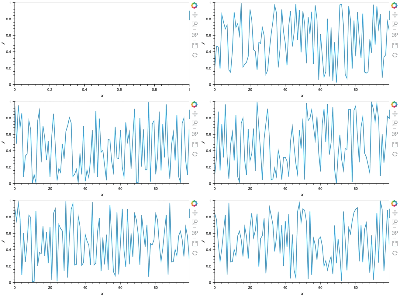 Since the callback is non-blocking we can continue working in the notebook and execute other cells. Once we're done we can stop the callback by calling ``cb.stop()``.
```python
cb.stop()
```
## Real examples
Using the ``Pipe`` and ``Buffer`` streams we can create complex streaming plots very easily. In addition to the toy examples we presented in this guide it is worth looking at looking at some of the examples using real, live, streaming data.
* The [streaming_psutil](http://holoviews.org/gallery/apps/bokeh/streaming_psutil.html) bokeh app is one such example which display CPU and memory information using the ``psutil`` library (install with ``pip install psutil`` or ``conda install psutil``)
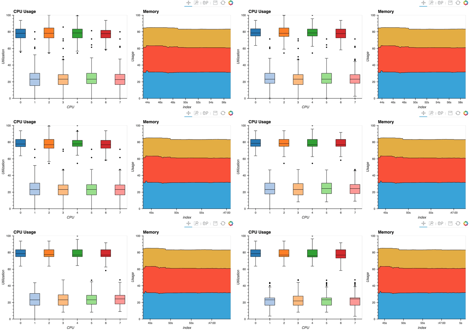 As you can see, streaming data works like streams in HoloViews in general, flexibly handling changes over time under either explicit control or governed by some external data source.
 Having set up this ``VectorField`` tied to a ``Pipe`` we can start pushing data to it varying the orientation of the VectorField:
```python
x,y = np.mgrid[-10:11,-10:11] * 0.1
sine_rings = np.sin(x**2+y**2)*np.pi+np.pi
exp_falloff = 1/np.exp((x**2+y**2)/8)
for i in np.linspace(0, 1, 25):
time.sleep(0.1)
pipe.send((x,y,sine_rings*i, exp_falloff))
```
This approach of using an element constructor directly does not allow you to use anything other than the default key and value dimensions. One simple workaround for this limitation is to use ``functools.partial`` as demonstrated in the **Controlling the length section** below.
Since ``Pipe`` is completely general and the data can be any custom type, it provides a completely general mechanism to stream structured or unstructured data. Due to this generality, ``Pipe`` does not offer some of the more complex features and optimizations available when using the ``Buffer`` stream described in the next section.
## ``Buffer``
While ``Pipe`` provides a general solution for piping arbitrary data to ``DynamicMap`` callback, ``Buffer`` on the other hand provides a very powerful means of working with streaming tabular data, defined as pandas dataframes, arrays or dictionaries of columns (as well as StreamingDataFrame, which we will cover later). ``Buffer`` automatically accumulates the last ``N`` rows of the tabular data, where ``N`` is defined by the ``length``.
The ability to accumulate data allows performing operations on a recent history of data, while plotting backends (such as bokeh) can optimize plot updates by sending just the latest patch. This optimization works only if the ``data`` object held by the ``Buffer`` is identical to the plotted ``Element`` data, otherwise all the data will be updated as normal.
#### A simple example: Brownian motion
To initialize a ``Buffer`` we have to provide an example dataset which defines the columns and dtypes of the data we will be streaming. Next we define the ``length`` to keep the last 100 rows of data. If the data is a DataFrame we can specify whether we will also want to use the ``DataFrame`` ``index``. In this case we will simply define that we want to plot a ``DataFrame`` of 'x' and 'y' positions and a 'count' as ``Points`` and ``Curve`` elements:
```python
example = pd.DataFrame({'x': [], 'y': [], 'count': []}, columns=['x', 'y', 'count'])
dfstream = Buffer(example, length=100, index=False)
curve_dmap = hv.DynamicMap(hv.Curve, streams=[dfstream])
point_dmap = hv.DynamicMap(hv.Points, streams=[dfstream])
```
After applying some styling we will display an ``Overlay`` of the dynamic ``Curve`` and ``Points``
```python
(curve_dmap * point_dmap).opts(
opts.Points(color='count', line_color='black', size=5, padding=0.1, xaxis=None, yaxis=None),
opts.Curve(line_width=1, color='black'))
```
 Now that we have set up the ``Buffer`` and defined a ``DynamicMap`` to plot the data we can start pushing data to it. We will define a simple function which simulates brownian motion by accumulating x, y positions. We can ``send`` data through the ``hv.streams.Buffer`` directly.
```python
def gen_brownian():
x, y, count = 0, 0, 0
while True:
x += np.random.randn()
y += np.random.randn()
count += 1
yield pd.DataFrame([(x, y, count)], columns=['x', 'y', 'count'])
brownian = gen_brownian()
for i in range(200):
dfstream.send(next(brownian))
```
Finally we can clear the data on the stream and plot using the ``clear`` method:
```python
dfstream.clear()
```
Note that when using the ``Buffer`` stream the view will always follow the current range of the data by default, by setting ``buffer.following=False`` or passing following as an argument to the constructor this behavior may be disabled.
## Using the Streamz library
Now that we have discovered what ``Pipe`` and ``Buffer`` can do it's time to show how you can use them together with the ``streamz`` library. Although HoloViews does not depend on ``streamz`` and you can use the streaming functionality without needing to learn about it, the two libraries work well together, allowing you to build pipelines to manage continuous streams of data. Streamz is easy to use for simple tasks, but also supports complex pipelines that involve branching, joining, flow control, feedback and more. Here we will mostly focus on connecting streamz output to ``Pipe`` and then ``Buffer`` so for more details about the streamz API, consult the [streamz documentation](https://streamz.readthedocs.io/en/latest/).
#### Using ``streamz.Stream`` together with ``Pipe``
Let's start with a fairly simple example:
1. Declare a ``streamz.Stream`` and a ``Pipe`` object and connect them into a pipeline into which we can push data.
2. Use a ``sliding_window`` of 10, which will first wait for 10 sets of stream updates to accumulate. At that point and for every subsequent update, it will apply ``pd.concat`` to combine the most recent 10 updates into a new dataframe.
3. Use the ``sink`` method on the ``streamz.Stream`` to ``send`` the resulting collection of 10 updates to ``Pipe``.
4. Declare a ``DynamicMap`` that takes the sliding window of concatenated DataFrames and displays it using a ``Scatter`` Element.
5. Color the ``Scatter`` points by their 'count' and set a range, then display:
```python
point_source = streamz.Stream()
pipe = Pipe(data=pd.DataFrame({'x': [], 'y': [], 'count': []}))
point_source.sliding_window(20).map(pd.concat).sink(pipe.send) # Connect streamz to the Pipe
scatter_dmap = hv.DynamicMap(hv.Scatter, streams=[pipe])
```
After set up our streaming pipeline we can again display it:
```python
scatter_dmap.opts(bgcolor='black', color='count', ylim=(-4, 4), show_legend=False)
```
 There is now a pipeline, but initially this plot will be empty, because no data has been sent to it. To see the plot update, let's use the ``emit`` method of ``streamz.Stream`` to send small chunks of random pandas ``DataFrame``s to our plot:
```python
for i in range(100):
df = pd.DataFrame({'x': np.random.rand(100), 'y': np.random.randn(100), 'count': i},
columns=['x', 'y', 'count'])
point_source.emit(df)
```
#### Using StreamingDataFrame and StreamingSeries
The streamz library provides ``StreamingDataFrame`` and ``StreamingSeries`` as a powerful way to easily work with live sources of tabular data. This makes it perfectly suited to work with ``Buffer``. With the ``StreamingDataFrame`` we can easily stream data, apply computations such as cumulative and rolling statistics and then visualize the data with HoloViews.
The ``streamz.dataframe`` module provides a ``Random`` utility that generates a ``StreamingDataFrame`` that emits random data with a certain frequency at a specified interval. The ``example`` attribute lets us see the structure and dtypes of the data we can expect:
```python
simple_sdf = streamz.dataframe.Random(freq='10ms', interval='100ms')
print(simple_sdf.index)
simple_sdf.example.dtypes
```
Since the ``StreamingDataFrame`` provides a pandas-like API, we can specify operations on the data directly. In this example we subtract a fixed offset and then compute the cumulative sum, giving us a randomly drifting timeseries. We can then pass the x-values of this dataframe to the HoloViews ``Buffer`` and supply ``hv.Curve`` as the ``DynamicMap`` callback to stream the data into a HoloViews ``Curve`` (with the default key and value dimensions):
```python
sdf = (simple_sdf-0.5).cumsum()
hv.DynamicMap(hv.Curve, streams=[Buffer(sdf.x)]).opts(width=500, show_grid=True)
```
 The ``Random`` StreamingDataFrame will asynchronously emit events, driving the visualization forward, until it is explicitly stopped, which we can do by calling the ``stop`` method.
```python
simple_sdf.stop()
```
#### Making use of the ``StreamingDataFrame`` API
So far we have only computed the cumulative sum, but the ``StreamingDataFrame`` actually has an extensive API that lets us run a broad range of streaming computations on our data. For example, let's apply a rolling mean to our x-values with a window of 500ms and overlay it on top of the 'raw' data:
```python
source_df = streamz.dataframe.Random(freq='5ms', interval='100ms')
sdf = (source_df-0.5).cumsum()
raw_dmap = hv.DynamicMap(hv.Curve, streams=[Buffer(sdf.x)])
smooth_dmap = hv.DynamicMap(hv.Curve, streams=[Buffer(sdf.x.rolling('500ms').mean())])
(raw_dmap.relabel('raw') * smooth_dmap.relabel('smooth')).opts(
opts.Curve(width=500, show_grid=True))
```
 ```python
source_df.stop()
```
#### Customizing elements with ``functools.partial``
In this notebook we have avoided defining custom functions for ``DynamicMap`` by simply supplying the element class and using the element constructor instead. Although this works well for examples, it often won't generalize to real-life situations, because you don't have an opportunity to use anything other than the default dimensions. One simple way to get around this limitation is to use ``functools.partial``:
```python
from functools import partial
```
Now you can now easily create an inline callable that creates an element with custom key and value dimensions by supplying them to ``partial`` in the form ``partial(hv.Element, kdims=[...], vdims=[...])``. In the next section, we will see an example of this pattern using ``hv.BoxWhisker``.
#### Controlling the length
By default the ``Buffer`` accumulates a ``length`` of 1000 samples. In many cases this may be excessive, but we can specify a shorter (or longer) length value to control how much history we accumulate, often depending on the element type.
In the following example, a custom ``length`` is used together with a ``partial`` wrapping ``hv.BoxWhisker`` in order to display a cumulative sum generated from a stream of random dataframes:
```python
multi_source = streamz.dataframe.Random(freq='50ms', interval='500ms')
sdf = (multi_source-0.5).cumsum()
hv.DynamicMap(hv.Table, streams=[Buffer(sdf.x, length=10)]) +\
hv.DynamicMap(partial(hv.BoxWhisker, kdims=[], vdims='x'), streams=[Buffer(sdf.x, length=100)])
```
```python
source_df.stop()
```
#### Customizing elements with ``functools.partial``
In this notebook we have avoided defining custom functions for ``DynamicMap`` by simply supplying the element class and using the element constructor instead. Although this works well for examples, it often won't generalize to real-life situations, because you don't have an opportunity to use anything other than the default dimensions. One simple way to get around this limitation is to use ``functools.partial``:
```python
from functools import partial
```
Now you can now easily create an inline callable that creates an element with custom key and value dimensions by supplying them to ``partial`` in the form ``partial(hv.Element, kdims=[...], vdims=[...])``. In the next section, we will see an example of this pattern using ``hv.BoxWhisker``.
#### Controlling the length
By default the ``Buffer`` accumulates a ``length`` of 1000 samples. In many cases this may be excessive, but we can specify a shorter (or longer) length value to control how much history we accumulate, often depending on the element type.
In the following example, a custom ``length`` is used together with a ``partial`` wrapping ``hv.BoxWhisker`` in order to display a cumulative sum generated from a stream of random dataframes:
```python
multi_source = streamz.dataframe.Random(freq='50ms', interval='500ms')
sdf = (multi_source-0.5).cumsum()
hv.DynamicMap(hv.Table, streams=[Buffer(sdf.x, length=10)]) +\
hv.DynamicMap(partial(hv.BoxWhisker, kdims=[], vdims='x'), streams=[Buffer(sdf.x, length=100)])
```
 Here the given stream ``sdf`` is being consumed by a table showing a short length (where only the items visible in the table need to be kept), along with a plot computing averages and variances over a longer length (100 items).
#### Updating multiple cells
Since a ``StreamingDataFrame`` will emit data until it is stopped, we can subscribe multiple plots across different cells to the same stream. Here, let's add a ``Scatter`` plot of the same data stream as in the preceding cell:
```python
hv.DynamicMap(hv.Scatter, streams=[Buffer(sdf.x)]).redim.label(x='value', index='time')
```
 Here we let the ``Scatter`` elements use the column names from the supplied ``DataFrames`` which are relabelled using the ``redim`` method. Stopping the stream will now stop updates to all three of these DynamicMaps:
```python
multi_source.stop()
```
## Operations over streaming data
As we discovered above, the ``Buffer`` lets us set a ``length``, which defines how many rows we want to accumulate. We can use this to our advantage and apply an operation over this length window. In this example we declare a ``Dataset`` and then apply the ``histogram`` operation to compute a ``Histogram`` over the specified ``length`` window:
```python
hist_source = streamz.dataframe.Random(freq='5ms', interval='100ms')
sdf = (hist_source-0.5).cumsum()
dmap = hv.DynamicMap(hv.Dataset, streams=[Buffer(sdf.x, length=500)])
hv.operation.histogram(dmap, dimension='x')
```
 ```python
hist_source.stop()
```
#### Datashading
The same approach will also work for the datashader operation letting us datashade the entire ``length`` window even if we make it very large such as 1 million samples:
```python
from holoviews.operation.datashader import datashade
from bokeh.palettes import Blues8
large_source = streamz.dataframe.Random(freq='100us', interval='200ms')
sdf = (large_source-0.5).cumsum()
dmap = hv.DynamicMap(hv.Curve, streams=[Buffer(sdf.x, length=1000000)])
datashade(dmap, streams=[hv.streams.PlotSize], cnorm='linear', cmap=list(Blues8)).opts(width=600)
```
```python
hist_source.stop()
```
#### Datashading
The same approach will also work for the datashader operation letting us datashade the entire ``length`` window even if we make it very large such as 1 million samples:
```python
from holoviews.operation.datashader import datashade
from bokeh.palettes import Blues8
large_source = streamz.dataframe.Random(freq='100us', interval='200ms')
sdf = (large_source-0.5).cumsum()
dmap = hv.DynamicMap(hv.Curve, streams=[Buffer(sdf.x, length=1000000)])
datashade(dmap, streams=[hv.streams.PlotSize], cnorm='linear', cmap=list(Blues8)).opts(width=600)
```
 ```python
large_source.stop()
```
## Asynchronous updates using the tornado ``IOLoop``
In most cases, instead of pushing updates manually from the same Python process, you'll want the object to update asynchronously as new data arrives. Since both Jupyter and Bokeh server run on [tornado](http://www.tornadoweb.org/en/stable/), we can use the tornado ``IOLoop`` in both cases to define a non-blocking co-routine that can push data to our stream whenever it is ready. The ``PeriodicCallback`` makes this approach very simple, we simply define a function which will be called periodically with a timeout defined in milliseconds. Once we have declared the callback we can call ``start`` to begin emitting events:
```python
from tornado.ioloop import PeriodicCallback
from tornado import gen
count = 0
buffer = Buffer(np.zeros((0, 2)), length=50)
@gen.coroutine
def f():
global count
count += 1
buffer.send(np.array([[count, np.random.rand()]]))
cb = PeriodicCallback(f, 100)
cb.start()
hv.DynamicMap(hv.Curve, streams=[buffer]).opts(padding=0.1, width=600)
```
```python
large_source.stop()
```
## Asynchronous updates using the tornado ``IOLoop``
In most cases, instead of pushing updates manually from the same Python process, you'll want the object to update asynchronously as new data arrives. Since both Jupyter and Bokeh server run on [tornado](http://www.tornadoweb.org/en/stable/), we can use the tornado ``IOLoop`` in both cases to define a non-blocking co-routine that can push data to our stream whenever it is ready. The ``PeriodicCallback`` makes this approach very simple, we simply define a function which will be called periodically with a timeout defined in milliseconds. Once we have declared the callback we can call ``start`` to begin emitting events:
```python
from tornado.ioloop import PeriodicCallback
from tornado import gen
count = 0
buffer = Buffer(np.zeros((0, 2)), length=50)
@gen.coroutine
def f():
global count
count += 1
buffer.send(np.array([[count, np.random.rand()]]))
cb = PeriodicCallback(f, 100)
cb.start()
hv.DynamicMap(hv.Curve, streams=[buffer]).opts(padding=0.1, width=600)
```
 Since the callback is non-blocking we can continue working in the notebook and execute other cells. Once we're done we can stop the callback by calling ``cb.stop()``.
```python
cb.stop()
```
## Real examples
Using the ``Pipe`` and ``Buffer`` streams we can create complex streaming plots very easily. In addition to the toy examples we presented in this guide it is worth looking at looking at some of the examples using real, live, streaming data.
* The [streaming_psutil](http://holoviews.org/gallery/apps/bokeh/streaming_psutil.html) bokeh app is one such example which display CPU and memory information using the ``psutil`` library (install with ``pip install psutil`` or ``conda install psutil``)
 As you can see, streaming data works like streams in HoloViews in general, flexibly handling changes over time under either explicit control or governed by some external data source.