
text
stringlengths 5
22M
| id
stringlengths 12
177
| metadata
dict | __index_level_0__
int64 0
1.37k
|
|---|---|---|---|
const axios = require('axios')
const fs = require('fs')
const pjson = require('../package.json')
const { convertData, convertNum } = require('../src/float-utils-node.js')
const CollaborativeTrainer64 = artifacts.require("./CollaborativeTrainer64")
const DataHandler64 = artifacts.require("./data/DataHandler64")
const Classifier = artifacts.require("./classification/SparsePerceptron")
const Stakeable64 = artifacts.require("./incentive/Stakeable64")
module.exports = async function (deployer) {
if (deployer.network === 'skipMigrations') {
return
}
// Information to persist to the database.
const name = "IMDB Review Sentiment Classifier"
const description = "A simple IMDB sentiment analysis model."
const encoder = 'IMDB vocab'
const modelInfo = {
name,
description,
accuracy: '0.829',
modelType: 'Classifier64',
encoder,
}
const toFloat = 1E9
// Low default times for testing.
const refundTimeS = 15
const anyAddressClaimWaitTimeS = 20
const ownerClaimWaitTimeS = 20
// Weight for deposit cost in wei.
const costWeight = 1E15
const data = fs.readFileSync('./src/ml-models/imdb-sentiment-model.json', 'utf8')
const model = JSON.parse(data)
const { classifications } = model
const weights = convertData(model.weights, web3, toFloat)
const initNumWords = 250
const numWordsPerUpdate = 250
console.log(`Deploying IMDB model with ${weights.length} weights.`)
const intercept = convertNum(model.intercept || model.bias, web3, toFloat)
const learningRate = convertNum(model.learningRate, web3, toFloat)
console.log(`Deploying DataHandler.`)
return deployer.deploy(DataHandler64).then(dataHandler => {
console.log(` Deployed data handler to ${dataHandler.address}.`)
return deployer.deploy(Stakeable64,
refundTimeS,
ownerClaimWaitTimeS,
anyAddressClaimWaitTimeS,
costWeight
).then(incentiveMechanism => {
console.log(` Deployed incentive mechanism to ${incentiveMechanism.address}.`)
console.log(`Deploying classifier.`)
return deployer.deploy(Classifier,
classifications, weights.slice(0, initNumWords), intercept, learningRate,
{ gas: 7.9E6 }).then(async classifier => {
console.log(` Deployed classifier to ${classifier.address}.`)
for (let i = initNumWords; i < weights.length; i += numWordsPerUpdate) {
await classifier.initializeWeights(i, weights.slice(i, i + numWordsPerUpdate),
{ gas: 7.9E6 })
console.log(` Added ${i + numWordsPerUpdate} weights.`)
}
console.log(`Deploying collaborative trainer contract.`)
return deployer.deploy(CollaborativeTrainer64,
name, description, encoder,
dataHandler.address,
incentiveMechanism.address,
classifier.address
).then(instance => {
console.log(` Deployed IMDB collaborative classifier to ${instance.address}.`)
return Promise.all([
dataHandler.transferOwnership(instance.address),
incentiveMechanism.transferOwnership(instance.address),
classifier.transferOwnership(instance.address),
]).then(() => {
modelInfo.address = instance.address
return axios.post(`${pjson.proxy}api/models`, modelInfo).then(() => {
console.log("Added model to the database.")
}).catch(err => {
if (process.env.CI !== "true" && process.env.REACT_APP_ENABLE_SERVICE_DATA_STORE === 'true') {
// It is okay to fail adding the model in CI but otherwise it should work.
console.error("Error adding model to the database.")
console.error(err)
throw err
}
})
})
})
})
})
})
}
| 0xDeCA10B/demo/client/migrations/2_deploy_sentiment_classifier.js/0 | {
"file_path": "0xDeCA10B/demo/client/migrations/2_deploy_sentiment_classifier.js",
"repo_id": "0xDeCA10B",
"token_count": 1284
} | 0 |
import Button from '@material-ui/core/Button'
import CircularProgress from '@material-ui/core/CircularProgress'
import Container from '@material-ui/core/Container'
import IconButton from '@material-ui/core/IconButton'
import Link from '@material-ui/core/Link'
import List from '@material-ui/core/List'
import ListItem from '@material-ui/core/ListItem'
import ListItemSecondaryAction from '@material-ui/core/ListItemSecondaryAction'
import ListItemText from '@material-ui/core/ListItemText'
import Modal from '@material-ui/core/Modal'
import Paper from '@material-ui/core/Paper'
import { withStyles } from '@material-ui/core/styles'
import Typography from '@material-ui/core/Typography'
import ClearIcon from '@material-ui/icons/Clear'
import DeleteIcon from '@material-ui/icons/Delete'
import { withSnackbar } from 'notistack'
import PropTypes from 'prop-types'
import React from 'react'
import update from 'immutability-helper'
import { checkStorages } from '../components/storageSelector'
import { getNetworkType } from '../getWeb3'
import { OnlineSafetyValidator } from '../safety/validator'
import { DataStoreFactory } from '../storage/data-store-factory'
import { BASE_TITLE } from '../title'
const styles = theme => ({
descriptionDiv: {
// Indent a bit to better align with text in the list.
marginLeft: theme.spacing(1),
marginRight: theme.spacing(1),
},
button: {
marginTop: 20,
marginBottom: 20,
marginLeft: 10,
},
spinnerDiv: {
textAlign: 'center',
marginTop: theme.spacing(2),
},
listDiv: {
marginTop: theme.spacing(2),
},
nextButtonContainer: {
textAlign: 'end',
},
removeModal: {
display: 'flex',
alignItems: 'center',
justifyContent: 'center',
},
removePaper: {
border: '2px solid lightgrey',
padding: '8px',
'box-shadow': 'lightgrey',
},
})
class ModelList extends React.Component {
constructor(props) {
super(props)
this.validator = new OnlineSafetyValidator()
this.storages = DataStoreFactory.getAll()
this.storageAfterAddress = {}
this.state = {
loadingModels: true,
numModelsRemaining: 0,
models: [],
permittedStorageTypes: [],
}
this.nextModels = this.nextModels.bind(this)
this.RemoveItemModal = this.RemoveItemModal.bind(this)
}
componentDidMount = async () => {
document.title = BASE_TITLE
checkStorages(this.storages).then(permittedStorageTypes => {
permittedStorageTypes = permittedStorageTypes.filter(storageType => storageType !== undefined)
this.setState({ permittedStorageTypes }, () => {
this.updateModels().then(() => {
// These checks are done after `updateModels`, otherwise a cycle of refreshes is triggered somehow.
if (typeof window !== "undefined" && window.ethereum) {
window.ethereum.on('accountsChanged', _accounts => { window.location.reload() })
window.ethereum.on('chainChanged', _chainId => { window.location.reload() })
}
})
})
})
}
notify(...args) {
return this.props.enqueueSnackbar(...args)
}
dismissNotification(...args) {
return this.props.closeSnackbar(...args)
}
nextModels() {
this.setState({
loadingModels: true,
models: [],
numModelsRemaining: 0
}, this.updateModels)
}
async updateModels() {
// TODO Also get valid contracts that the account has already interacted with.
// TODO Filter out models that are not on this network.
const networkType = await getNetworkType()
const limit = 6
return Promise.all(this.state.permittedStorageTypes.map(storageType => {
const afterId = this.storageAfterAddress[storageType]
return this.storages[storageType].getModels(afterId, limit).then(response => {
const newModels = response.models
const { remaining } = response
newModels.forEach(model => {
model.restrictInfo = storageType !== 'local' && !this.validator.isPermitted(networkType, model.address)
model.metaDataLocation = storageType
})
if (newModels.length > 0) {
this.storageAfterAddress[storageType] = newModels[newModels.length - 1].address
}
this.setState(prevState => ({
models: prevState.models.concat(newModels),
numModelsRemaining: prevState.numModelsRemaining + remaining
}))
}).catch(err => {
this.notify(`Could not get ${storageType} models`, { variant: 'error' })
console.error(`Could not get ${storageType} models.`)
console.error(err)
})
})).finally(_ => {
this.setState({ loadingModels: false })
})
}
handleStartRemove(removeItem, removeItemIndex) {
this.setState({
removeItem,
removeItemIndex
})
}
handleCancelRemove() {
this.setState({
removeItem: undefined,
removeItemIndex: undefined,
})
}
handleRemove() {
const { removeItem, removeItemIndex } = this.state
this.storages.local.removeModel(removeItem).then(response => {
const { success } = response
if (success) {
// Remove from the list.
this.setState({
removeItem: undefined,
removeItemIndex: undefined,
models: update(this.state.models, { $splice: [[removeItemIndex, 1]] }),
})
this.notify("Removed", { variant: "success" })
} else {
throw new Error("Error removing.")
}
}).catch(err => {
console.error("Error removing.")
console.error(err)
this.notify("Error while removing", { variant: "error" })
})
}
RemoveItemModal() {
return (<Modal
aria-labelledby="remove-item-modal-title"
aria-describedby="remove-modal-title"
open={this.state.removeItem !== undefined}
onClose={() => { this.setState({ removeItem: undefined }) }}
className={this.props.classes.removeModal}
>
<Paper className={this.props.classes.removePaper}>
<Typography component="p" id="remove-choice-modal-title">
{this.state.removeItem &&
`Are you sure you would like to remove "${this.state.removeItem.name || this.state.removeItem.description}" from your local meta-data? This does not remove the model from the blockchain.`}
</Typography>
<Button className={this.props.classes.button} variant="outlined" //color="primary"
size="small" onClick={() => this.handleRemove()}>
Remove <DeleteIcon color="error" />
</Button>
<Button className={this.props.classes.button} variant="outlined" //color="primary"
size="small" onClick={() => this.handleCancelRemove()}>
Cancel <ClearIcon color="action" />
</Button>
</Paper>
</Modal>)
}
render() {
const listItems = this.state.models.map((m, index) => {
const url = `/model?${m.id ? `modelId=${m.id}&` : ''}address=${m.address}&metaDataLocation=${m.metaDataLocation}&tab=predict`
const allowRemoval = m.metaDataLocation === 'local'
return (
<ListItem key={`model-${index}`} button component="a" href={url}>
<ListItemText primary={m.restrictInfo ? `(name hidden) Address: ${m.address}` : m.name}
secondary={m.accuracy && `Accuracy: ${(m.accuracy * 100).toFixed(1)}%`} />
{/* For accessibility: keep secondary action even when disabled so that the <li> is used. */}
<ListItemSecondaryAction>
{allowRemoval &&
<IconButton edge="end" aria-label="delete" onClick={(event) => {
this.handleStartRemove(m, index); event.preventDefault()
}} >
<DeleteIcon />
</IconButton>
}
</ListItemSecondaryAction>
</ListItem>
)
})
const serviceStorageEnabled = this.state.permittedStorageTypes.indexOf('service') > 0
return (
<div>
<this.RemoveItemModal />
<Container>
<div className={this.props.classes.descriptionDiv}>
<Typography variant="h5" component="h5">
Welcome to Sharing Updatable Models
</Typography>
<Typography component="p">
Here you will find models stored on a blockchain that you can interact with.
Models are added to this list if you have recorded them on your device in this browser
{serviceStorageEnabled ? " or if they are listed on a centralized database" : ""}.
</Typography>
<Typography component="p">
You can deploy your own model <Link href='/add'>here</Link> or use an already deployed model by filling in the information <Link href='/addDeployedModel'>here</Link>.
</Typography>
</div>
{this.state.loadingModels ?
<div className={this.props.classes.spinnerDiv}>
<CircularProgress size={100} />
</div>
: listItems.length > 0 ?
<div className={this.props.classes.listDiv}>
{this.state.numModelsRemaining > 0 &&
<div className={this.props.classes.nextButtonContainer}>
<Button className={this.props.classes.button} variant="outlined" color="primary"
onClick={this.nextModels}
>
Next
</Button>
</div>
}
<Paper>
<List className={this.props.classes.list}>
{listItems}
</List>
</Paper>
{this.state.numModelsRemaining > 0 &&
<div className={this.props.classes.nextButtonContainer}>
<Button className={this.props.classes.button} variant="outlined" color="primary"
onClick={this.nextModels}
>
Next
</Button>
</div>
}
</div>
:
<div className={this.props.classes.descriptionDiv}>
<Typography component="p">
You do not have any models listed.
</Typography>
</div>
}
</Container>
</div>
)
}
}
ModelList.propTypes = {
classes: PropTypes.object.isRequired,
}
export default withSnackbar(withStyles(styles)(ModelList))
| 0xDeCA10B/demo/client/src/containers/modelList.js/0 | {
"file_path": "0xDeCA10B/demo/client/src/containers/modelList.js",
"repo_id": "0xDeCA10B",
"token_count": 3691
} | 1 |
/**
* Possible types of encoders.
* The string values can be stored in smart contracts on public blockchains so do not make changes to the values.
* Changing the casing of a value should be fine.
*/
export enum Encoder {
// Simple encoders:
None = "none",
Mult1E9Round = "Multiply by 1E9, then round",
// Hash encoders:
MurmurHash3 = "MurmurHash3",
// More complicated encoders:
ImdbVocab = "IMDB vocab",
MobileNetV2 = "MobileNetV2",
USE = "universal sentence encoder",
}
export function normalizeEncoderName(encoderName: string): string {
if (!encoderName) {
return encoderName
}
return encoderName.toLocaleLowerCase('en')
}
| 0xDeCA10B/demo/client/src/encoding/encoder.ts/0 | {
"file_path": "0xDeCA10B/demo/client/src/encoding/encoder.ts",
"repo_id": "0xDeCA10B",
"token_count": 213
} | 2 |
const fs = require('fs')
const path = require('path')
const mobilenet = require('@tensorflow-models/mobilenet')
const tf = require('@tensorflow/tfjs-node')
const { createCanvas, loadImage } = require('canvas')
const { normalize1d } = require('../tensor-utils-node')
const dataPath = path.join(__dirname, './seefood')
const POSITIVE_CLASS = "HOT DOG"
const NEGATIVE_CLASS = "NOT HOT DOG"
const INTENTS = {
'hot_dog': POSITIVE_CLASS,
'not_hot_dog': NEGATIVE_CLASS,
}
// Normalize each sample like what will happen in production to avoid changing the centroid by too much.
const NORMALIZE_EACH_EMBEDDING = true
// Reduce the size of the embeddings.
const REDUCE_EMBEDDINGS = false
const EMB_SIZE = 1280
const EMB_REDUCTION_FACTOR = REDUCE_EMBEDDINGS ? 4 : 1
// Classifier type can be: ncc/perceptron
const args = process.argv.slice(2)
const CLASSIFIER_TYPE = args.length > 0 ? args[0] : 'perceptron'
console.log(`Training a ${CLASSIFIER_TYPE} classifier.`)
// Perceptron Classifier Config
// Take only the top features.
const PERCEPTRON_NUM_FEATS = 400
// Sort of like regularization but it does not converge.
// Probably because it ruins the Perceptron assumption of updating weights.
const NORMALIZE_PERCEPTRON_WEIGHTS = false
let learningRate = 1
const LEARNING_RATE_CHANGE_FACTOR = 0.8618
const LEARNING_RATE_CUTTING_PERCENT_OF_BEST = 0.8618
const MAX_STABILITY_COUNT = 3
const PERCENT_OF_TRAINING_SET_TO_FIT = 0.99
const classes = {
[POSITIVE_CLASS]: +1,
[NEGATIVE_CLASS]: -1,
}
// Nearest Centroid Classifier Config
// Normalizing the centroid didn't change performance by much.
// It was slightly worse for HOT_DOG accuracy.
const NORMALIZE_CENTROID = false
let embeddingCache
const embeddingCachePath = path.join(__dirname, 'embedding_cache.json')
if (fs.existsSync(embeddingCachePath)) {
try {
embeddingCache = fs.readFileSync(embeddingCachePath, 'utf8')
embeddingCache = JSON.parse(embeddingCache)
console.debug(`Loaded ${Object.keys(embeddingCache).length} cached embeddings.`)
} catch (error) {
console.error("Error loading embedding cache.\nWill create a new one.")
console.error(error)
embeddingCache = {}
}
} else {
embeddingCache = {}
}
// Useful for making the embedding smaller.
// This did not change the accuracy by much.
if (EMB_SIZE % EMB_REDUCTION_FACTOR !== 0) {
throw new Error("The embedding reduction factor is not a multiple of the embedding size.")
}
const EMB_MAPPER =
tf.tidy(_ => {
const mapper = tf.fill([EMB_SIZE / EMB_REDUCTION_FACTOR, EMB_SIZE], 0, 'int32')
const buffer = mapper.bufferSync()
for (let i = 0; i < mapper.shape[0]; ++i) {
for (let j = 0; j < EMB_REDUCTION_FACTOR; ++j) {
buffer.set(1, i, 2 * i + j)
}
}
return buffer.toTensor()
})
/**
* @param {string} sample The relative path from `dataPath` for the image.
* @returns The embedding for the image. Shape has 1 dimension.
*/
async function getEmbedding(sample) {
let result = embeddingCache[sample]
if (result !== undefined) {
result = tf.tensor1d(result)
} else {
const img = await loadImage(path.join(dataPath, sample))
const canvas = createCanvas(img.width, img.height)
const ctx = canvas.getContext('2d')
ctx.drawImage(img, 0, 0)
const emb = await encoder.infer(canvas, { embedding: true })
if (emb.shape[1] !== EMB_SIZE) {
throw new Error(`Expected embedding to have ${EMB_SIZE} dimensions. Got shape: ${emb.shape}.`)
}
result = tf.tidy(_ => {
let result = emb.gather(0)
embeddingCache[sample] = result.arraySync()
if (REDUCE_EMBEDDINGS) {
result = EMB_MAPPER.dot(result)
}
return result
})
emb.dispose()
}
if (NORMALIZE_EACH_EMBEDDING) {
const normalizedResult = normalize1d(result)
result.dispose()
result = normalizedResult
}
return result
}
/**
* Shuffles array in place.
* @param {Array} a items An array containing the items.
*/
// From https://stackoverflow.com/a/6274381/1226799
function shuffle(a) {
for (let i = a.length - 1; i > 0; i--) {
const j = Math.floor(Math.random() * (i + 1));
[a[i], a[j]] = [a[j], a[i]]
}
return a
}
async function predict(model, sample) {
switch (CLASSIFIER_TYPE) {
case 'ncc':
return await predictNearestCentroidModel(model, sample)
case 'perceptron':
return await predictPerceptron(model, sample)
default:
throw new Error(`Unrecognized classifierType: "${CLASSIFIER_TYPE}"`)
}
}
async function evaluate(model) {
const evalStats = []
const evalIntents = Object.entries(INTENTS)
for (let i = 0; i < evalIntents.length; ++i) {
const [intent, expectedIntent] = evalIntents[i]
const stats = {
intent: expectedIntent,
recall: undefined,
numCorrect: 0,
confusion: {},
}
const pathPrefix = path.join('test', intent)
const dataDir = path.join(dataPath, pathPrefix)
const samples = fs.readdirSync(dataDir)
console.log(`Evaluating with ${samples.length} samples for ${INTENTS[intent]}.`)
for (let i = 0; i < samples.length; ++i) {
if (i % Math.round(samples.length / 5) == 0) {
// console.log(` ${expectedIntent}: ${(100 * i / samples.length).toFixed(1)}% (${i}/${samples.length})`);
}
const prediction = await predict(model, path.join(pathPrefix, samples[i]))
if (prediction === expectedIntent) {
stats.numCorrect += 1
} else {
if (!(prediction in stats.confusion)) {
stats.confusion[prediction] = 0
}
stats.confusion[prediction] += 1
}
}
stats.recall = stats.numCorrect / samples.length
evalStats.push(stats)
// console.log(` ${expectedIntent}: Done evaluating.`);
}
console.log(`NORMALIZE_EACH_EMBEDDING: ${NORMALIZE_EACH_EMBEDDING}`)
console.log(`NORMALIZE_PERCEPTRON_WEIGHTS: ${NORMALIZE_PERCEPTRON_WEIGHTS}`)
switch (CLASSIFIER_TYPE) {
case 'ncc':
console.log(`normalizeCentroid: ${NORMALIZE_CENTROID}`)
break
case 'perceptron':
console.log(`learningRate: ${learningRate}`)
break
default:
throw new Error(`Unrecognized classifierType: "${CLASSIFIER_TYPE}"`)
}
// Compute precision.
Object.values(INTENTS).forEach(intent => {
evalStats.forEach(stats => {
if (stats.intent === intent) {
let numFalsePositives = 0
evalStats.forEach(otherStats => {
if (otherStats.intent !== intent) {
if (otherStats.confusion[intent] !== undefined) {
numFalsePositives += otherStats.confusion[intent]
}
}
})
stats.precision = stats.numCorrect / (stats.numCorrect + numFalsePositives)
stats.f1 = 2 / (1 / stats.precision + 1 / stats.recall)
}
})
})
console.log(JSON.stringify(evalStats, null, 2))
let f1HarmonicMean = 0
for (let i = 0; i < evalStats.length; ++i) {
f1HarmonicMean += 1 / evalStats[i].f1
}
f1HarmonicMean = evalStats.length / f1HarmonicMean
console.log(`f1 harmonic mean: ${f1HarmonicMean.toFixed(3)}`)
}
// Nearest Centroid Classifier Section
async function getCentroid(intent) {
const pathPrefix = path.join('train', intent)
const dataDir = path.join(dataPath, pathPrefix)
const samples = fs.readdirSync(dataDir)
console.log(`Training with ${samples.length} samples for ${INTENTS[intent]}.`)
const allEmbeddings = []
for (let i = 0; i < samples.length; ++i) {
if (i % 100 == 0) {
console.log(` ${INTENTS[intent]}: ${(100 * i / samples.length).toFixed(1)}% (${i}/${samples.length})`)
}
const emb = await getEmbedding(path.join(pathPrefix, samples[i]))
allEmbeddings.push(emb.expandDims())
}
console.log(` ${INTENTS[intent]}: Done getting embeddings.`)
const centroid = tf.tidy(() => {
const allEmbTensor = tf.concat(allEmbeddings)
if (allEmbTensor.shape[0] !== samples.length) {
throw new Error(`Some embeddings are missing: allEmbTensor.shape[0] !== samples.length: ${allEmbTensor.shape[0]} !== ${samples.length}`)
}
let centroid = allEmbTensor.mean(axis = 0)
if (NORMALIZE_CENTROID) {
centroid = normalize1d(centroid)
}
return centroid.arraySync()
})
allEmbeddings.forEach(emb => emb.dispose())
return {
centroid,
dataCount: samples.length,
}
}
function getNearestCentroidModel() {
return new Promise((resolve, reject) => {
Promise.all(Object.keys(INTENTS).map(getCentroid))
.then(async centroidInfos => {
const model = { intents: {} }
Object.values(INTENTS).forEach((intent, i) => {
model.intents[intent] = centroidInfos[i]
})
const modelPath = path.join(__dirname, 'classifier-centroids.json')
console.log(`Saving centroids to "${modelPath}".`)
model.type = 'nearest centroid classifier'
fs.writeFileSync(modelPath, JSON.stringify(model))
resolve(model)
}).catch(reject)
})
}
async function predictNearestCentroidModel(model, sample) {
let minDistance = Number.MAX_VALUE
let result
const emb = await getEmbedding(sample)
tf.tidy(() => {
Object.entries(model.intents).forEach(([intent, centroidInfo]) => {
const centroid = tf.tensor1d(centroidInfo.centroid)
const distance = centroid.sub(emb).pow(2).sum()
if (distance.less(minDistance).dataSync()[0]) {
result = intent
minDistance = distance
}
})
})
emb.dispose()
return result
}
// Perceptron Section
async function getPerceptronModel() {
return new Promise(async (resolve, reject) => {
// Load data.
const samples = []
Object.keys(INTENTS).forEach(intent => {
const pathPrefix = path.join('train', intent)
const dataDir = path.join(dataPath, pathPrefix)
const samplesForClass = fs.readdirSync(dataDir).map(sample => {
return {
classification: INTENTS[intent],
path: path.join(pathPrefix, sample)
}
})
samples.push(...samplesForClass)
})
const model = {
bias: 0,
}
// Initialize the weights.
console.log(` Training with ${EMB_SIZE} weights.`)
model.weights = new Array(EMB_SIZE)
for (let j = 0; j < model.weights.length; ++j) {
// Can initialize randomly with `Math.random() - 0.5` but it doesn't seem to make much of a difference.
// model.weights[j] = 0;
model.weights[j] = Math.random() - 0.5
}
model.weights = tf.tidy(_ => {
return normalize1d(tf.tensor1d(model.weights))
})
let numUpdates, bestNumUpdatesBeforeLearningRateChange
let epoch = 0
let stabilityCount = 0
do {
if (model.weights !== undefined && NORMALIZE_PERCEPTRON_WEIGHTS) {
// Sort of like regularization.
model.weights = normalize1d(model.weights)
}
numUpdates = 0
shuffle(samples)
for (let i = 0; i < samples.length; ++i) {
if (i % Math.round(samples.length / 4) == 0) {
// console.log(` training: ${(100 * i / samples.length).toFixed(1)}% (${i}/${samples.length})`);
}
const sample = samples[i]
const emb = await getEmbedding(sample.path)
const { classification } = sample
const prediction = await predictPerceptron(model, emb)
if (prediction !== classification) {
numUpdates += 1
const sign = classes[classification]
model.weights = tf.tidy(_ => { return model.weights.add(emb.mul(sign * learningRate)) })
}
emb.dispose()
}
console.log(`Training epoch: ${epoch.toString().padStart(4, '0')}: numUpdates: ${numUpdates}`)
if (numUpdates === 0) {
// There cannot be any more updates.
break
}
epoch += 1
if (bestNumUpdatesBeforeLearningRateChange !== undefined &&
numUpdates < bestNumUpdatesBeforeLearningRateChange * LEARNING_RATE_CUTTING_PERCENT_OF_BEST) {
learningRate *= LEARNING_RATE_CHANGE_FACTOR
console.debug(` Changed learning rate to: ${learningRate.toFixed(3)}`)
bestNumUpdatesBeforeLearningRateChange = numUpdates
}
if (bestNumUpdatesBeforeLearningRateChange === undefined) {
bestNumUpdatesBeforeLearningRateChange = numUpdates
}
if (numUpdates < Math.max(samples.length * (1 - PERCENT_OF_TRAINING_SET_TO_FIT), 1)) {
stabilityCount += 1
} else {
stabilityCount = 0
}
} while (stabilityCount < MAX_STABILITY_COUNT)
const modelPath = path.join(__dirname, 'classifier-perceptron.json')
console.log(`Saving Perceptron to "${modelPath}".`)
fs.writeFileSync(modelPath, JSON.stringify({
type: 'perceptron',
weights: model.weights.arraySync(),
classifications: [NEGATIVE_CLASS, POSITIVE_CLASS],
bias: model.bias
}))
resolve(model)
})
}
async function predictPerceptron(model, sample) {
let result
let emb = sample
if (typeof sample === 'string') {
emb = await getEmbedding(sample)
}
tf.tidy(() => {
if (model.featureIndices !== undefined) {
emb = emb.gather(model.featureIndices)
}
let prediction = model.weights.dot(emb)
prediction = prediction.add(model.bias)
if (prediction.greater(0).dataSync()[0]) {
result = POSITIVE_CLASS
} else {
result = NEGATIVE_CLASS
}
})
if (typeof sample === 'string') {
emb.dispose()
}
return result
}
async function main() {
global.encoder = await mobilenet.load(
{
version: 2,
alpha: 1,
}
)
let model
switch (CLASSIFIER_TYPE) {
case 'ncc':
model = await getNearestCentroidModel()
break
case 'perceptron':
model = await getPerceptronModel()
break
default:
throw new Error(`Unrecognized classifierType: "${CLASSIFIER_TYPE}"`)
}
await evaluate(model)
fs.writeFileSync(embeddingCachePath, JSON.stringify(embeddingCache))
console.debug(`Wrote embedding cache to \"${embeddingCachePath}\" with ${Object.keys(embeddingCache).length} cached embeddings.`)
if (CLASSIFIER_TYPE === 'perceptron' && PERCEPTRON_NUM_FEATS !== EMB_SIZE) {
console.log(`Reducing weights to ${PERCEPTRON_NUM_FEATS} dimensions.`)
model.featureIndices = tf.tidy(_ => {
return tf.abs(model.weights).topk(PERCEPTRON_NUM_FEATS).indices
})
model.weights = tf.tidy(_ => {
return model.weights.gather(model.featureIndices)
})
const modelPath = path.join(__dirname, `classifier-perceptron-${PERCEPTRON_NUM_FEATS}.json`)
console.log(`Saving Perceptron with ${PERCEPTRON_NUM_FEATS} weights to "${modelPath}".`)
fs.writeFileSync(modelPath, JSON.stringify({
type: 'perceptron',
classifications: [NEGATIVE_CLASS, POSITIVE_CLASS],
featureIndices: model.featureIndices.arraySync(),
weights: model.weights.arraySync(),
bias: model.bias
}))
await evaluate(model)
}
}
main()
| 0xDeCA10B/demo/client/src/ml-models/hot_dog-not/train-classifier.js/0 | {
"file_path": "0xDeCA10B/demo/client/src/ml-models/hot_dog-not/train-classifier.js",
"repo_id": "0xDeCA10B",
"token_count": 5504
} | 3 |
import { DataStore, DataStoreHealthStatus, ModelInformation, ModelsResponse, OriginalData, RemoveResponse } from './data-store'
export class LocalDataStore implements DataStore {
errorOpening?: boolean
db?: IDBDatabase
private readonly dataStoreName = 'data'
private readonly modelStoreName = 'model'
constructor() {
const openRequest = indexedDB.open("database", 1)
openRequest.onerror = (event: any) => {
this.errorOpening = true
console.error("Could not open the database.")
console.error(event)
throw new Error("Could not open the database.")
}
openRequest.onsuccess = (event: any) => {
this.db = event.target.result
}
openRequest.onupgradeneeded = (event: any) => {
const db: IDBDatabase = event.target.result
// Index by transaction hash.
db.createObjectStore(this.dataStoreName, { keyPath: 'tx' })
const modelStore = db.createObjectStore(this.modelStoreName, { keyPath: 'address' })
modelStore.createIndex('address', 'address')
}
}
private checkOpened(timeout = 0): Promise<void> {
return new Promise((resolve, reject) => {
setTimeout(() => {
if (this.db) {
resolve()
} else if (this.errorOpening) {
reject(new Error("The database could not be opened."))
} else {
this.checkOpened(Math.min(500, 1.618 * timeout + 10))
.then(resolve)
.catch(reject)
}
}, timeout)
})
}
health(): Promise<DataStoreHealthStatus> {
return this.checkOpened().then(() => {
return new DataStoreHealthStatus(true)
})
}
async saveOriginalData(transactionHash: string, originalData: OriginalData): Promise<any> {
await this.checkOpened()
return new Promise((resolve, reject) => {
const transaction = this.db!.transaction(this.dataStoreName, 'readwrite')
transaction.onerror = reject
const dataStore = transaction.objectStore(this.dataStoreName)
const request = dataStore.add({ tx: transactionHash, text: originalData.text })
request.onerror = reject
request.onsuccess = resolve
})
}
async getOriginalData(transactionHash: string): Promise<OriginalData> {
await this.checkOpened()
return new Promise((resolve, reject) => {
const transaction = this.db!.transaction(this.dataStoreName, 'readonly')
transaction.onerror = reject
const dataStore = transaction.objectStore(this.dataStoreName)
const request = dataStore.get(transactionHash)
request.onerror = reject
request.onsuccess = (event: any) => {
const originalData = event.target.result
if (originalData === undefined) {
reject(new Error("Data not found."))
} else {
const { text } = originalData
resolve(new OriginalData(text))
}
}
})
}
async saveModelInformation(modelInformation: ModelInformation): Promise<any> {
await this.checkOpened()
return new Promise((resolve, reject) => {
const transaction = this.db!.transaction(this.modelStoreName, 'readwrite')
transaction.onerror = reject
const modelStore = transaction.objectStore(this.modelStoreName)
const request = modelStore.add(modelInformation)
request.onerror = reject
request.onsuccess = resolve
})
}
async getModels(afterAddress?: string, limit?: number): Promise<ModelsResponse> {
await this.checkOpened()
return new Promise((resolve, reject) => {
const transaction = this.db!.transaction(this.modelStoreName, 'readonly')
transaction.onerror = reject
const modelStore = transaction.objectStore(this.modelStoreName)
const index = modelStore.index('address')
const models: ModelInformation[] = []
if (afterAddress == null) {
afterAddress = ''
}
const open = true
const range = IDBKeyRange.lowerBound(afterAddress, open)
let count = 0
index.openCursor(range).onsuccess = (event: any) => {
const cursor = event.target.result
if (cursor && (limit == null || count++ < limit)) {
models.push(new ModelInformation(cursor.value))
cursor.continue()
} else {
const countRequest = index.count(range)
countRequest.onsuccess = () => {
const remaining = countRequest.result - models.length
resolve(new ModelsResponse(models, remaining))
}
}
}
})
}
async getModel(_modelId?: number, address?: string): Promise<ModelInformation> {
if (address === null || address === undefined) {
throw new Error("An address is required.")
}
await this.checkOpened()
return new Promise((resolve, reject) => {
const transaction = this.db!.transaction(this.modelStoreName, 'readonly')
transaction.onerror = reject
const modelStore = transaction.objectStore(this.modelStoreName)
const request = modelStore.get(address)
request.onerror = reject
request.onsuccess = (event: any) => {
const model = event.target.result
if (model === undefined) {
reject(new Error("Model not found."))
} else {
resolve(new ModelInformation(model))
}
}
})
}
async removeModel(modelInformation: ModelInformation): Promise<RemoveResponse> {
await this.checkOpened()
return new Promise((resolve, reject) => {
const transaction = this.db!.transaction(this.modelStoreName, 'readwrite')
transaction.onerror = reject
const modelStore = transaction.objectStore(this.modelStoreName)
const request = modelStore.delete(modelInformation.address)
request.onerror = reject
request.onsuccess = () => {
const success = true
resolve(new RemoveResponse(success))
}
})
}
}
| 0xDeCA10B/demo/client/src/storage/local-data-store.ts/0 | {
"file_path": "0xDeCA10B/demo/client/src/storage/local-data-store.ts",
"repo_id": "0xDeCA10B",
"token_count": 1893
} | 4 |
const Environment = require('jest-environment-jsdom')
/**
* A custom environment to set the TextEncoder that is required by TensorFlow.js.
*/
module.exports = class CustomTestEnvironment extends Environment {
// Following https://stackoverflow.com/a/57713960/1226799
async setup() {
await super.setup()
if (typeof this.global.TextEncoder === 'undefined') {
const { TextEncoder } = require('util')
this.global.TextEncoder = TextEncoder
}
if (typeof this.global.indexedDB === 'undefined') {
this.global.indexedDB = require('fake-indexeddb')
}
if (typeof this.global.IDBKeyRange === 'undefined') {
this.global.IDBKeyRange = require("fake-indexeddb/lib/FDBKeyRange")
}
if (typeof this.global.web3 === 'undefined') {
const Web3 = require('web3')
const truffleConfig = require('../truffle')
const networkConfig = truffleConfig.networks.development
this.global.web3 = new Web3(new Web3.providers.HttpProvider(`http://${networkConfig.host}:${networkConfig.port}`))
}
}
}
| 0xDeCA10B/demo/client/test/custom-test-env.js/0 | {
"file_path": "0xDeCA10B/demo/client/test/custom-test-env.js",
"repo_id": "0xDeCA10B",
"token_count": 356
} | 5 |
import random
import unittest
import numpy as np
from injector import Injector
from decai.simulation.contract.balances import Balances
from decai.simulation.contract.classification.classifier import Classifier
from decai.simulation.contract.classification.perceptron import PerceptronModule
from decai.simulation.contract.collab_trainer import CollaborativeTrainer, DefaultCollaborativeTrainerModule
from decai.simulation.contract.incentive.stakeable import StakeableImModule
from decai.simulation.contract.objects import Msg, RejectException, TimeMock
from decai.simulation.logging_module import LoggingModule
def _ground_truth(data):
return data[0] * data[2]
class TestCollaborativeTrainer(unittest.TestCase):
@classmethod
def setUpClass(cls):
inj = Injector([
DefaultCollaborativeTrainerModule,
LoggingModule,
PerceptronModule,
StakeableImModule,
])
cls.balances = inj.get(Balances)
cls.decai = inj.get(CollaborativeTrainer)
cls.time_method = inj.get(TimeMock)
cls.good_address = 'sender'
initial_balance = 1E6
cls.balances.initialize(cls.good_address, initial_balance)
msg = Msg(cls.good_address, cls.balances[cls.good_address])
X = np.array([
# Initialization Data
[0, 0, 0],
[1, 1, 1],
# Data to Add
[0, 0, 1],
[0, 1, 0],
[0, 1, 1],
[1, 0, 0],
[1, 0, 1],
[1, 1, 0],
])
y = np.array([_ground_truth(x) for x in X])
cls.decai.model.init_model(np.array([X[0, :], X[1, :]]),
np.array([y[0], y[1]]))
score = cls.decai.model.evaluate(X, y)
assert score != 1, "Model shouldn't fit the data yet."
# Add all data.
first_added_time = None
for i in range(X.shape[0]):
x = X[i]
cls.time_method.set_time(cls.time_method() + 1)
if first_added_time is None:
first_added_time = cls.time_method()
cls.decai.add_data(msg, x, y[i])
for _ in range(1000):
score = cls.decai.model.evaluate(X, y)
if score >= 1:
break
i = random.randint(0, X.shape[0] - 1)
x = X[i]
cls.time_method.set_time(cls.time_method() + 1)
cls.decai.add_data(msg, x, y[i])
assert score == 1, "Model didn't fit the data."
bal = cls.balances[msg.sender]
assert bal < initial_balance, "Adding data should have a cost."
# Make sure sender has some good data refunded so that they can report data later.
cls.time_method.set_time(cls.time_method() + cls.decai.im.refund_time_s + 1)
cls.decai.refund(msg, X[0], y[0], first_added_time)
assert cls.balances[msg.sender] > bal, "Refunding should return value."
def test_predict(self):
data = np.array([0, 1, 0])
correct_class = _ground_truth(data)
prediction = self.decai.model.predict(data)
self.assertEqual(prediction, correct_class)
def test_refund(self):
data = np.array([0, 2, 0])
correct_class = _ground_truth(data)
orig_address = "Orig"
bal = 1E5
self.balances.initialize(orig_address, bal)
msg = Msg(orig_address, 1E3)
self.time_method.set_time(self.time_method() + 1)
added_time = self.time_method()
self.decai.add_data(msg, data, correct_class)
self.assertLess(self.balances[orig_address], bal)
# Add same data from another address.
msg = Msg(self.good_address, 1E3)
self.time_method.set_time(self.time_method() + 1)
bal = self.balances[self.good_address]
self.decai.add_data(msg, data, correct_class)
self.assertLess(self.balances[self.good_address], bal)
# Original address refunds.
msg = Msg(orig_address, 1E3)
bal = self.balances[orig_address]
self.time_method.set_time(self.time_method() + self.decai.im.refund_time_s + 1)
self.decai.refund(msg, data, correct_class, added_time)
self.assertGreater(self.balances[orig_address], bal)
def test_report(self):
data = np.array([0, 0, 0])
correct_class = _ground_truth(data)
submitted_classification = 1 - correct_class
# Add bad data.
malicious_address = 'malicious'
self.balances.initialize(malicious_address, 1E6)
bal = self.balances[malicious_address]
msg = Msg(malicious_address, bal)
self.time_method.set_time(self.time_method() + 1)
added_time = self.time_method()
self.decai.add_data(msg, data, submitted_classification)
self.assertLess(self.balances[malicious_address], bal,
"Adding data should have a cost.")
self.time_method.set_time(self.time_method() + self.decai.im.refund_time_s + 1)
# Can't refund.
msg = Msg(malicious_address, self.balances[malicious_address])
try:
self.decai.refund(msg, data, submitted_classification, added_time)
self.fail("Should have failed.")
except RejectException as e:
self.assertEqual("The model doesn't agree with your contribution.", e.args[0])
bal = self.balances[self.good_address]
msg = Msg(self.good_address, bal)
self.decai.report(msg, data, submitted_classification, added_time, malicious_address)
self.assertGreater(self.balances[self.good_address], bal)
def test_report_take_all(self):
data = np.array([0, 0, 0])
correct_class = _ground_truth(data)
submitted_classification = 1 - correct_class
# Add bad data.
malicious_address = 'malicious_take_backer'
self.balances.initialize(malicious_address, 1E6)
bal = self.balances[malicious_address]
msg = Msg(malicious_address, bal)
self.time_method.set_time(self.time_method() + 1)
added_time = self.time_method()
self.decai.add_data(msg, data, submitted_classification)
self.assertLess(self.balances[malicious_address], bal,
"Adding data should have a cost.")
self.time_method.set_time(self.time_method() + self.decai.im.any_address_claim_wait_time_s + 1)
# Can't refund.
msg = Msg(malicious_address, self.balances[malicious_address])
try:
self.decai.refund(msg, data, submitted_classification, added_time)
self.fail("Should have failed.")
except RejectException as e:
self.assertEqual("The model doesn't agree with your contribution.", e.args[0])
bal = self.balances[malicious_address]
msg = Msg(malicious_address, bal)
self.decai.report(msg, data, submitted_classification, added_time, malicious_address)
self.assertGreater(self.balances[malicious_address], bal)
def test_reset(self):
inj = Injector([
LoggingModule,
PerceptronModule,
])
m = inj.get(Classifier)
X = np.array([
# Initialization Data
[0, 0, 0],
[1, 1, 1],
])
y = np.array([_ground_truth(x) for x in X])
m.init_model(X, y, save_model=True)
data = np.array([
[0, 0, 0],
[0, 0, 1],
[0, 1, 0],
[0, 1, 1],
[1, 0, 0],
[1, 0, 1],
[1, 1, 0],
[1, 1, 1],
])
original_predictions = [m.predict(x) for x in data]
labels = np.array([_ground_truth(x) for x in data])
for x, y in zip(data, labels):
m.update(x, y)
predictions_after_training = [m.predict(x) for x in data]
self.assertNotEqual(original_predictions, predictions_after_training)
m.reset_model()
new_predictions = [m.predict(x) for x in data]
self.assertEqual(original_predictions, new_predictions)
| 0xDeCA10B/simulation/decai/simulation/contract/classification/tests/test_perceptron.py/0 | {
"file_path": "0xDeCA10B/simulation/decai/simulation/contract/classification/tests/test_perceptron.py",
"repo_id": "0xDeCA10B",
"token_count": 3780
} | 6 |
import unittest
from typing import cast
from injector import Injector
from decai.simulation.data.data_loader import DataLoader
from decai.simulation.data.ttt_data_loader import TicTacToeDataLoader, TicTacToeDataModule
from decai.simulation.logging_module import LoggingModule
class TestTicTacToeDataLoader(unittest.TestCase):
@classmethod
def setUpClass(cls):
inj = Injector([
LoggingModule,
TicTacToeDataModule,
])
cls.ttt = inj.get(DataLoader)
assert isinstance(cls.ttt, TicTacToeDataLoader)
cls.ttt = cast(TicTacToeDataLoader, cls.ttt)
def test_classifications(self):
classifications = self.ttt.classifications()
assert classifications == ["(0, 0)", "(0, 1)", "(0, 2)",
"(1, 0)", "(1, 1)", "(1, 2)",
"(2, 0)", "(2, 1)", "(2, 2)"]
def test_boards(self):
(x_train, y_train), (x_test, y_test) = self.ttt.load_data()
assert x_train.shape[1] == self.ttt.width * self.ttt.length
assert set(x_train[x_train != 0]) == {1, -1}
assert x_test.shape[1] == self.ttt.width * self.ttt.length
assert set(x_test[x_test != 0]) == {1, -1}
assert set(y_train) <= set(range(9))
assert set(y_test) <= set(range(9))
| 0xDeCA10B/simulation/decai/simulation/data/tests/test_ttt_data_loader.py/0 | {
"file_path": "0xDeCA10B/simulation/decai/simulation/data/tests/test_ttt_data_loader.py",
"repo_id": "0xDeCA10B",
"token_count": 633
} | 7 |
# MIT License
# Copyright (c) Microsoft Corporation.
# Permission is hereby granted, free of charge, to any person obtaining a copy
# of this software and associated documentation files (the "Software"), to deal
# in the Software without restriction, including without limitation the rights
# to use, copy, modify, merge, publish, distribute, sublicense, and/or sell
# copies of the Software, and to permit persons to whom the Software is
# furnished to do so, subject to the following conditions:
# The above copyright notice and this permission notice shall be included in all
# copies or substantial portions of the Software.
# THE SOFTWARE IS PROVIDED "AS IS", WITHOUT WARRANTY OF ANY KIND, EXPRESS OR
# IMPLIED, INCLUDING BUT NOT LIMITED TO THE WARRANTIES OF MERCHANTABILITY,
# FITNESS FOR A PARTICULAR PURPOSE AND NONINFRINGEMENT. IN NO EVENT SHALL THE
# AUTHORS OR COPYRIGHT HOLDERS BE LIABLE FOR ANY CLAIM, DAMAGES OR OTHER
# LIABILITY, WHETHER IN AN ACTION OF CONTRACT, TORT OR OTHERWISE, ARISING FROM,
# OUT OF OR IN CONNECTION WITH THE SOFTWARE OR THE USE OR OTHER DEALINGS IN THE
# SOFTWARE
import torch
import torch.nn as nn
class DropPath(nn.Module):
def __init__(self, p=0.):
"""
Drop path with probability.
Parameters
----------
p : float
Probability of an path to be zeroed.
"""
super().__init__()
self.p = p
def forward(self, x):
if self.training and self.p > 0.:
keep_prob = 1. - self.p
# per data point mask
mask = torch.zeros((x.size(0), 1, 1, 1), device=x.device).bernoulli_(keep_prob)
return x / keep_prob * mask
return x
class PoolBN(nn.Module):
"""
AvgPool or MaxPool with BN. `pool_type` must be `max` or `avg`.
"""
def __init__(self, pool_type, C, kernel_size, stride, padding, affine=True):
super().__init__()
if pool_type.lower() == 'max':
self.pool = nn.MaxPool2d(kernel_size, stride, padding)
elif pool_type.lower() == 'avg':
self.pool = nn.AvgPool2d(kernel_size, stride, padding, count_include_pad=False)
else:
raise ValueError()
self.bn = nn.BatchNorm2d(C, affine=affine)
def forward(self, x):
out = self.pool(x)
out = self.bn(out)
return out
class StdConv(nn.Module):
"""
Standard conv: ReLU - Conv - BN
"""
def __init__(self, C_in, C_out, kernel_size, stride, padding, affine=True):
super().__init__()
self.net = nn.Sequential(
nn.ReLU(),
nn.Conv2d(C_in, C_out, kernel_size, stride, padding, bias=False),
nn.BatchNorm2d(C_out, affine=affine)
)
def forward(self, x):
return self.net(x)
class FacConv(nn.Module):
"""
Factorized conv: ReLU - Conv(Kx1) - Conv(1xK) - BN
"""
def __init__(self, C_in, C_out, kernel_length, stride, padding, affine=True):
super().__init__()
self.net = nn.Sequential(
nn.ReLU(),
nn.Conv2d(C_in, C_in, (kernel_length, 1), stride, padding, bias=False),
nn.Conv2d(C_in, C_out, (1, kernel_length), stride, padding, bias=False),
nn.BatchNorm2d(C_out, affine=affine)
)
def forward(self, x):
return self.net(x)
class DilConv(nn.Module):
"""
(Dilated) depthwise separable conv.
ReLU - (Dilated) depthwise separable - Pointwise - BN.
If dilation == 2, 3x3 conv => 5x5 receptive field, 5x5 conv => 9x9 receptive field.
"""
def __init__(self, C_in, C_out, kernel_size, stride, padding, dilation, affine=True):
super().__init__()
self.net = nn.Sequential(
nn.ReLU(),
nn.Conv2d(C_in, C_in, kernel_size, stride, padding, dilation=dilation, groups=C_in,
bias=False),
nn.Conv2d(C_in, C_out, 1, stride=1, padding=0, bias=False),
nn.BatchNorm2d(C_out, affine=affine)
)
def forward(self, x):
return self.net(x)
class SepConv(nn.Module):
"""
Depthwise separable conv.
DilConv(dilation=1) * 2.
"""
def __init__(self, C_in, C_out, kernel_size, stride, padding, affine=True):
super().__init__()
self.net = nn.Sequential(
DilConv(C_in, C_in, kernel_size, stride, padding, dilation=1, affine=affine),
DilConv(C_in, C_out, kernel_size, 1, padding, dilation=1, affine=affine)
)
def forward(self, x):
return self.net(x)
class FactorizedReduce(nn.Module):
"""
Reduce feature map size by factorized pointwise (stride=2).
"""
def __init__(self, C_in, C_out, affine=True):
super().__init__()
self.relu = nn.ReLU()
self.conv1 = nn.Conv2d(C_in, C_out // 2, 1, stride=2, padding=0, bias=False)
self.conv2 = nn.Conv2d(C_in, C_out // 2, 1, stride=2, padding=0, bias=False)
self.bn = nn.BatchNorm2d(C_out, affine=affine)
def forward(self, x):
x = self.relu(x)
out = torch.cat([self.conv1(x), self.conv2(x[:, :, 1:, 1:])], dim=1)
out = self.bn(out)
return out
| AI-System/Labs/AdvancedLabs/Lab8/nas/ops.py/0 | {
"file_path": "AI-System/Labs/AdvancedLabs/Lab8/nas/ops.py",
"repo_id": "AI-System",
"token_count": 2296
} | 8 |
<!--Copyright © Microsoft Corporation. All rights reserved.
适用于[License](https://github.com/microsoft/AI-System/blob/main/LICENSE)版权许可-->
# 12.3 人工智能服务安全与隐私
- [12.3 人工智能服务安全与隐私](#122-人工智能训练安全与隐私)
- [12.3.1 服务时安全](#1221-服务时安全)
- [12.3.2 服务时的用户隐私](#1222-服务时的用户隐私)
- [12.3.3 服务时的模型隐私](#1223-服务时的模型隐私)
- [小结与讨论](#小结与讨论)
- [参考文献](#参考文献)
本节介绍人工智能服务时的安全与隐私问题及缓解方法。这些问题涉及到人工智能推理的完整性与机密性,反映了可信人工智能推理系统的重要性。
## 12.2.1 服务时安全
对于一个部署好的深度学习服务,推理系统通常将模型参数存储在内存中。但是,内存在长期的使用后是可能发生错误的,例如其中的一些比特发生了反转。Guanpeng Li 等人[<sup>[1]</sup>](#softerror)在 2017 年研究发现深度学习推理系统常常使用的高性能硬件更容易出现这种内存错误(如果这种错误可以通过重启消除,则称为软错误),而软错误会在深度神经网络中传导,导致模型的结果出错。这种现象如果被恶意攻击者利用,就可以通过故障注入攻击(Fault Injection Attack)来篡改内存中存储的模型参数,从而影响模型的行为。Sanghyun Hong 等人[<sup>[2]</sup>](#braindamage)在 2019 年提出如果精心选择,一个比特翻转就能让模型的精度下降超过
90%。他们还通过 Rowhammer 故障注入攻击(恶意程序通过大量反复读写内存的特定位置来使目标内存位置的数据出错)成功让运行在同一台机器上的受害模型下降 99% 的分类精度。这种攻击的危害之处在于它无需攻击者物理访问目标设备,只需要软件干扰就能让模型失效。如果模型部署在手机、自动驾驶汽车等不受部署者控制的终端设备上,可能会造成更严重的安全问题。
对于这种攻击,最简单的缓解方式是使用量化后的模型,因为量化后的模型参数是以整数存储的,而整数对于比特翻转的敏感性比浮点数小。但是,Adnan Siraj Rakin 等人[<sup>[3]</sup>](#bitflip)在 2019 年提出了一种针对量化深度神经网络的攻击,利用梯度下降的思想来搜索模型中最敏感的几个参数。例如,对于一个有九千多万比特参数的量化深度神经网络,找到并翻转其中最敏感的 13 个比特,成功地使其分类精度降到只有 0.1%。
由此可见,对于攻击者来说深度神经网络是非常脆弱的,这颠覆了之前很多人的观点——之前认为深度神经网络是健壮的,一些微小的改动并不会产生大的影响。对此弱点,比较好的缓解方法是将模型部署到拥有纠错功能的内存(ECC 内存)中,因为 ECC 内存会在硬件中自动维护纠错码(Error Correction Code),其能够对于每个字节自动更正一比特的错误,或者发现但不更正(可以通知系统通过重启解决)两比特的错误。这是基于汉明码(Hamming Code)来实现的,下面简单介绍:
<style>
table {
margin: auto;
}
</style>
<center>表 12.3.1 带附加奇偶校验位的 (7, 4)-汉明码</center>
| |p1|p2|d1|p3|d2|d3|d4|p4|
|---|---|---|---|---|---|---|---|---|
|p1|x| |x| |x| |x| |
|p2| |x|x| | |x|x| |
|p3| | | |x|x|x|x| |
|p4|x|x|x|x|x|x|x|x|
如果要编码 4 位数据 $(d_1, d_2, d_3, d_4)$,需要增加 3 位奇偶校验位 $(p_1, p_2, p_3)$ 以及附加的一位奇偶校验位 $p_4$,总共 8 位排列成 $(p_1, p_2, d_1, p_3, d_2, d_3, d_4, p_4)$ 的顺序,构成所谓“带附加奇偶校验位的汉明码”(其前 7 位称为“(7, 4)-汉明码”,最后一位为附加的奇偶校验位 $p_4$)。奇偶校验位的取值应该使所覆盖的位置(即表中的 x 所在的位置)中有且仅有**偶数个** 1,即:
$$
p_1=d_1\oplus d_2\oplus d_4 \\
p_2=d_1\oplus d_3\oplus d_4 \\
p_3=d_2\oplus d_3\oplus d_4 \\
p_4=p_1\oplus p_2\oplus d_1\oplus p_3\oplus d_2\oplus d_3\oplus d_4
$$
其中 $\oplus$ 表示异或。这样,如果出现了位翻转错误,无论是 $(p_1, p_2, d_1, p_3, d_2, d_3, d_4, p_4)$ 中的哪一位出错,都可以通过上面的公式推算出错的是哪一个,并且进行更正。通过验证上面的公式是否成立,也可以确定是否发生了(两位以内的)错误。目前流行的 ECC 内存一般采用的是带附加奇偶校验位的 (71,64)-汉明码,即每 64 比特的数据需要 72 比特进行编码。
## 12.2.2 服务时的用户隐私
深度学习服务时最直接的隐私就是用户隐私。服务以用户传来的数据作为输入,那么这些数据可能会直接暴露给服务方,服务方能够看到、甚至收集这些输入数据(以及最后的输出数据),在很多时候这是可能侵犯到用户隐私的。例如使用医疗模型进行辅助诊断时,用户很可能并不希望自己的输入数据被模型拥有者或者运营商知晓。
这时候,可以使用 12.2.2 节中提到过的安全多方计算技术来保护用户隐私,同时完成深度神经网络的推理计算。2017 年,Jian Liu 等人[<sup>[4]</sup>](#minionn)设计了针对深度神经网络推理计算的安全多方计算协议,这个协议的参与方是用户和服务方两方,在个算过程中用户的输入和中间结果都是保持着秘密共享的状态,因此服务方无法知道关于用户数据的信息。虽然安全多方计算可能有成千上万倍的开销,但对于小规模的模型推理计算(例如 LeNet-5)来说可以做到一秒以内的延迟了。近几年来,有大量的研究工作致力于提升安全多方计算的效率。目前,最新的工作[<sup>[5]</sup>](#cheetah)可以在十几秒的时间内完成 ResNet32 的安全推理计算。
除了安全多方计算之外,同态加密和可信执行环境都是进行安全推理计算的常用隐私计算技术。其目的与安全多方计算一样,都是保护模型推理时的输入(以及输出)数据隐私,使服务方在不知道输入的情况下完成计算。用同态加密做深度神经网络计算的代表工作是 2016 年由 Ran Gilad-Bachrach 等人提出的 CryptoNets[<sup>[6]</sup>](#cryptonets):通过对输入数据进行同态加密,可以将密文发送给服务方并让服务方在密文上做计算,最终将密文结果发回用户,用户用私钥对其解密得到计算结果。CryptoNets 使用的[微软 SEAL 库](https://github.com/microsoft/SEAL)也是目前最为广泛使用的同态加密库。然而,同态加密也有非常大的开销,目前来看其计算开销比安全多方计算的计算开销更大,但通信开销更小。此外,同态加密有一个与安全多方计算相似的局限:对于加法、乘法的支持很好,计算开销也比较小;但对于其他类型的计算(如深度神经网络中的非线性激活函数)的支持并不好,计算开销非常大,因此为了提升性能会用多项式来进行近似,从而有计算开销与计算精度(近似的程度)之间的权衡问题。
相比于安全多方计算、同态加密的性能瓶颈,基于可信执行环境的方案有着很最高的性能。可信执行环境是处理器在内存中隔离出的一个安全的区域,由处理器硬件保证区域内数据的机密性、完整性。以 Intel 处理器的 SGX(Software Guard Extensions)技术为例,处理器中的内存控制器保证其他进程无法访问或篡改可信执行环境(Intel 称之为 enclave)中的代码和数据,并且保证这些数据在存储、传输过程中都是加密保护的,密钥只掌握在处理器硬件中;只有使用这些数据时,才会在处理器内部对其解密并使用。基于这种技术,只要将模型推理系统部署在服务器的可信执行环境中,就能保护用户数据的隐私,因为这种技术让服务方自己都不能获取可信执行环境中的数据。尽管早期的 SGX 有可用容量的问题(不到 128 MB),但这个问题可以通过软件设计[<sup>[7]</sup>](#occ)或硬件设计[<sup>[8]</sup>](#graviton)的方法进行改善。目前,更先进的 TEE 架构设计已经出现在了商用产品上:Intel 的 Ice Lake 架构的服务器端 CPU 已经支持了 SGX 2,大大扩展了可用容量;NVIDIA 最新的 H100 处理器成为了首个提供 TEE 的 GPU。可信执行环境的缺点是开发难度高,又存在引入额外信任的问题——这一方案只有在信任处理器制造方的情况下才是安全的。近年来针对可信执行环境的攻击也非常多,暴露了许多安全缺陷[<sup>[9]</sup>](#sok)[<sup>[10]</sup>](#survey),说明这一信任并不一定是可靠的。
以上三种隐私计算技术都各有利弊,需要根据实际场景的特点进行选择和适配。这些领域还在快速发展中,相信未来一定会有高效、易用的解决方案,让保护用户隐私的深度学习服务能更广泛地部署在人们的日常生活中。
## 12.2.3 服务时的模型隐私
上一小节主要站在用户的角度,探讨了输入数据的隐私保护问题。事实上,站在开发者以及模型拥有者的角度,模型也是一种高度敏感的数据。考虑到模型在实际使用中可能涉及到知识产权问题,以及训练该模型所需要的大量数据和大量计算成本,保证其机密性对于深度学习服务来说是个重要问题。本小节将讨论跟模型数据保护相关的攻击。
一种最常见的针对模型数据的攻击就是模型窃取攻击(Model Stealing Attack)。模型窃取有两种方式,第一种是直接窃取,即通过直接攻克模型的开发、存储或部署环境,获得原模型的拷贝;第二种是间接窃取,通过不断调用服务提供的 API(Application Programming Interface),重构出一个与原模型等效或近似等效的模型。前者的例子有 Lejla Batina 等人在 2019 年提出的通过侧信道攻击进行的模型窃取[<sup>[11]</sup>](#sidechannel)。而人工智能安全领域关注的模型窃取攻击通常属于第二种,因为这种攻击看上去并没有违背深度学习服务系统的完整性与机密性,只通过 API 调用这一看起来正常的手段就窃取了模型;而且,即使使用了 12.2.2 节中的隐私计算技术保护了用户隐私,但攻击者(伪装成普通用户)仍然知道自己的输入和服务返回的结果,因此隐私计算对于防御这种攻击无能为力。
最简单的模型窃取攻击是针对线性模型 $f(x)=\textrm{sigmoid}(wx+b)$ 的:通过选取足够多个不同的 $x$ 并调用服务 API 得到相应的 $y$,将其组成一个以 $w$ 和 $b$ 为未知数的线性方程组,就可以解出该线性方程组,得到模型参数 $w$ 和 $b$。2016 年,Florian Tramèr 等人将这种方法扩展到了多层的神经网络上:由于深度神经网络的非线性层,组成的方程组不再是一个线性方程组,没有解析解,所以改用优化方法来求解近似解[<sup>[12]</sup>](#extract)。这种方法本质上就像把深度学习服务当作一个标注机,然后利用它来进行监督学习。
不过需要注意的是,调用服务 API 是有成本的,因为这些服务往往是按次收费的。所以,如果所需的调用次数太多导致成本过高,攻击就变得没有意义了。近几年关于模型窃取攻击的一大研究方向就是如何提升攻击的效率,即如何用更少的询问次数来得到与目标模型等效或近似等效的模型。2020 年 Matthew Jagielski 等人优化了学习策略,通过半监督学习的方式大大提升了攻击的效率[<sup>[13]</sup>](#extract2)。同时,他们还讨论了另一种攻击目标:精准度,即能否像攻击线性模型那样准确地恢复出模型的参数。他们注意到采用 ReLU 激活函数的深度神经网络其实是一个分段线性函数,因此可以在各个线性区域内确定分类面的位置,从而恢复出模型参数。同样是 2020 年,Nicholas Carlini 等人通过密码分析学的方法进行模型提取攻击,也精确恢复了深度神经网络的参数[<sup>[14]</sup>](#extract3)。事实上,如果模型参数被精确提取出来了,那除了模型参数泄露之外还会有更大的安全问题:这时模型对于攻击者来说变成白盒了,因此更容易发起成员推断攻击和模型反向攻击了(见 12.1.2),从而导致训练模型时所用的训练数据的隐私泄露。
如何保护模型的隐私呢?由于模型窃取攻击往往需要大量请求服务 API,可以通过限制请求次数来进行缓解。另一种防御方法是去检测模型窃取攻击:Mika Juuti 等人在 2019 年提出模型窃取攻击时发出的请求和正常的请求有不同的特征,可以由此判断什么样的请求是的攻击者发起的请求[<sup>[15]</sup>](#prada)。还有一种防御的策略是事后溯源以及追责:如果模型被窃取,假如可以验证模型的所有权,那么可以通过法律手段制裁攻击者。这种策略可以通过模型水印技术(见 12.2.1)来实现。
## 小结与讨论
本小节主要围绕深度学习的服务安全与隐私问题,讨论了故障注入攻击、模型提取攻击等攻击技术,服务时的用户隐私与模型隐私问题,以及 ECC 内存、安全多方计算、同态加密、可信执行环境等防御技术。
看完本章内容后,我们可以思考以下几点问题:
- 纠错码检查错误和纠错的具体过程是什么?如何用硬件实现?效率如何?
- 不同隐私计算技术的异同是什么?
- 能否利用可信执行环境来防止模型窃取攻击?
## 参考文献
<div id=softerror></div>
1. Guanpeng Li, Siva Kumar Sastry Hari, Michael B. Sullivan, Timothy Tsai, Karthik Pattabiraman, Joel S. Emer, and Stephen W. Keckler. 2017. [Understanding Error Propagation in Deep Learning Neural Network (DNN) Accelerators and Applications](https://doi.org/10.1145/3126908.3126964). In International Conference for High Performance Computing, Networking, Storage and Analysis (SC), 8:1-8:12.
<div id=braindamage></div>
2. Sanghyun Hong, Pietro Frigo, Yigitcan Kaya, Cristiano Giuffrida, and Tudor Dumitras. 2019. [Terminal Brain Damage: Exposing the Graceless Degradation in Deep Neural Networks Under Hardware Fault Attacks](https://www.usenix.org/conference/usenixsecurity19/presentation/hong). In USENIX Security Symposium, 497–514.
<div id=bitflip></div>
3. Adnan Siraj Rakin, Zhezhi He, and Deliang Fan. 2019. [Bit-Flip Attack: Crushing Neural Network With Progressive Bit Search](https://doi.org/10.1109/ICCV.2019.00130). In IEEE International Conference on Computer Vision (ICCV), 1211–1220.
<div id=minionn></div>
4. Jian Liu, Mika Juuti, Yao Lu, and N. Asokan. 2017. [Oblivious Neural Network Predictions via MiniONN Transformations](https://doi.org/10.1145/3133956.3134056). In ACM Conference on Computer and Communications Security (CCS), 619–631.
<div id=cheetah></div>
5. Zhicong Huang, Wen-jie Lu, Cheng Hong, and Jiansheng Ding. 2022. [Cheetah: Lean and Fast Secure Two-Party Deep Neural Network Inference](https://www.usenix.org/system/files/sec22fall_huang-zhicong.pdf). In USENIX Security Symposium.
<div id=cryptonets></div>
6. Ran Gilad-Bachrach, Nathan Dowlin, Kim Laine, Kristin E. Lauter, Michael Naehrig, and John Wernsing. 2016. [CryptoNets: Applying Neural Networks to Encrypted Data with High Throughput and Accuracy](http://proceedings.mlr.press/v48/gilad-bachrach16.html). In International Conference on Machine Learning (ICML), 201–210.
<div id=occ></div>
7. Taegyeong Lee, Zhiqi Lin, Saumay Pushp, Caihua Li, Yunxin Liu, Youngki Lee, Fengyuan Xu, Chenren Xu, Lintao Zhang, and Junehwa Song. 2019. [Occlumency: Privacy-preserving Remote Deep-learning Inference Using SGX](https://doi.org/10.1145/3300061.3345447). In International Conference on Mobile Computing and Networking (MobiCom), 46:1-46:17.
<div id=graviton></div>
8. Stavros Volos, Kapil Vaswani, and Rodrigo Bruno. 2018. [Graviton: Trusted Execution Environments on GPUs](https://www.usenix.org/conference/osdi18/presentation/volos). In USENIX Symposium on Operating Systems Design and Implementation (OSDI), 681–696.
<div id=sok></div>
9. David Cerdeira, Nuno Santos, Pedro Fonseca, and Sandro Pinto. 2020. [SoK: Understanding the Prevailing Security Vulnerabilities in TrustZone-assisted TEE Systems](https://doi.org/10.1109/SP40000.2020.00061). In IEEE Symposium on Security and Privacy (S&P), 1416–1432.
<div id=sok></div>
10. Shufan Fei, Zheng Yan, Wenxiu Ding, and Haomeng Xie. 2021. [Security Vulnerabilities of SGX and Countermeasures: A Survey](https://doi.org/10.1145/3456631). ACM Computing Surveys 54, 6 (2021), 126:1-126:36.
<div id=sidechannel></div>
11. Lejla Batina, Shivam Bhasin, Dirmanto Jap, and Stjepan Picek. 2019. [CSI NN: Reverse Engineering of Neural Network Architectures Through Electromagnetic Side Channel](https://www.usenix.org/conference/usenixsecurity19/presentation/batina). In USENIX Security Symposium, 515–532.
<div id=extract></div>
12. Florian Tramèr, Fan Zhang, Ari Juels, Michael K. Reiter, and Thomas Ristenpart. 2016. [Stealing Machine Learning Models via Prediction APIs](https://www.usenix.org/conference/usenixsecurity16/technical-sessions/presentation/tramer). In USENIX Security Symposium, 601–618.
<div id=extract2></div>
13. Matthew Jagielski, Nicholas Carlini, David Berthelot, Alex Kurakin, and Nicolas Papernot. 2020. [High Accuracy and High Fidelity Extraction of Neural Networks](https://www.usenix.org/conference/usenixsecurity20/presentation/jagielski). In USENIX Security Symposium, 1345–1362.
<div id=extract3></div>
14. Nicholas Carlini, Matthew Jagielski, and Ilya Mironov. 2020. [Cryptanalytic Extraction of Neural Network Models](https://doi.org/10.1007/978-3-030-56877-1_7). In Annual International Cryptology Conference (CRYPTO), 189–218.
<div id=prada></div>
15. Mika Juuti, Sebastian Szyller, Samuel Marchal, and N. Asokan. 2019. [PRADA: Protecting Against DNN Model Stealing Attacks](https://doi.org/10.1109/EuroSP.2019.00044). In European Symposium on Security and Privacy (EuroS&P), 512–527.
| AI-System/Textbook/第12章-人工智能安全与隐私/12.3-人工智能服务安全与隐私.md/0 | {
"file_path": "AI-System/Textbook/第12章-人工智能安全与隐私/12.3-人工智能服务安全与隐私.md",
"repo_id": "AI-System",
"token_count": 11352
} | 9 |
<!--Copyright © Microsoft Corporation. All rights reserved.
适用于[License](https://github.com/microsoft/AI-System/blob/main/LICENSE)版权许可-->
## 2.3 解决回归问题
本小节主要围绕解决回归问题中的各个环节和知识点展开,包含提出问题,万能近似定力,定义神经网络结构,前向计算和反向传播等内容。
- [2.3 解决回归问题](#23-解决回归问题)
- [2.3.1 提出问题](#231-提出问题)
- [2.3.2 万能近似定理](#232-万能近似定理)
- [2.3.3 定义神经网络结构](#233-定义神经网络结构)
- [输入层](#输入层)
- [权重矩阵W1/B1](#权重矩阵w1b1)
- [隐层](#隐层)
- [权重矩阵W2/B2](#权重矩阵w2b2)
- [输出层](#输出层)
- [2.3.4 前向计算](#234-前向计算)
- [隐层](#隐层-1)
- [输出层](#输出层-1)
- [损失函数](#损失函数)
- [代码](#代码)
- [2.3.5 反向传播](#235-反向传播)
- [求损失函数对输出层的反向误差](#求损失函数对输出层的反向误差)
- [求W2的梯度](#求w2的梯度)
- [求B2的梯度](#求b2的梯度)
- [求损失函数对隐层的反向误差](#求损失函数对隐层的反向误差)
- [代码](#代码-1)
- [2.3.6 运行结果](#236-运行结果)
- [小结与讨论](#小结与讨论)
- [参考文献](#参考文献)
### 2.3.1 提出问题
前面的正弦函数,看上去是非常有规律的,也许单层神经网络很容易就做到了。如果是更复杂的曲线,单层神经网络还能轻易做到吗?比如图9-2所示的样本点和表9-2的所示的样本值,如何使用神经网络方法来拟合这条曲线?
<img src="./img/Sample.png"/>
图 2.3.1 复杂曲线样本可视化
表 2.3.1 复杂曲线样本数据
|样本|x|y|
|---|---|---|
|1|0.606|-0.113|
|2|0.129|-0.269|
|3|0.582|0.027|
|...|...|...|
|1000|0.199|-0.281|
上面这条“蛇形”曲线,实际上是由下面这个公式添加噪音后生成的:
$$y=0.4x^2 + 0.3x\sin(15x) + 0.01\cos(50x)-0.3$$
我们特意把数据限制在[0,1]之间,避免做归一化的麻烦。要是觉得这个公式还不够复杂,大家可以用更复杂的公式去自己做试验。
以上问题可以叫做非线性回归,即自变量X和因变量Y之间不是线性关系。常用的传统的处理方法有线性迭代法、分段回归法、迭代最小二乘法等。在神经网络中,解决这类问题的思路非常简单,就是使用带有一个隐层的两层神经网络。
### 2.3.2 万能近似定理
万能近似定理(universal approximation theorem) $^{[1]}$,是深度学习最根本的理论依据。它证明了在给定网络具有足够多的隐藏单元的条件下,配备一个线性输出层和一个带有任何“挤压”性质的激活函数(如Sigmoid激活函数)的隐藏层的前馈神经网络,能够以任何想要的误差量近似任何从一个有限维度的空间映射到另一个有限维度空间的Borel可测的函数。
前馈网络的导数也可以以任意好地程度近似函数的导数。
万能近似定理其实说明了理论上神经网络可以近似任何函数。但实践上我们不能保证学习算法一定能学习到目标函数。即使网络可以表示这个函数,学习也可能因为两个不同的原因而失败:
1. 用于训练的优化算法可能找不到用于期望函数的参数值;
2. 训练算法可能由于过拟合而选择了错误的函数。
根据“没有免费的午餐”定理,说明了没有普遍优越的机器学习算法。前馈网络提供了表示函数的万能系统,在这种意义上,给定一个函数,存在一个前馈网络能够近似该函数。但不存在万能的过程既能够验证训练集上的特殊样本,又能够选择一个函数来扩展到训练集上没有的点。
总之,具有单层的前馈网络足以表示任何函数,但是网络层可能大得不可实现,并且可能无法正确地学习和泛化。在很多情况下,使用更深的模型能够减少表示期望函数所需的单元的数量,并且可以减少泛化误差。
### 2.3.3 定义神经网络结构
根据万能近似定理的要求,我们定义一个两层的神经网络,输入层不算,一个隐藏层,含3个神经元,一个输出层。图 2.3.2 显示了此次用到的神经网络结构。
<img src="./img/nn1.png" />
图 2.3.2 单入单出的双层神经网络
为什么用3个神经元呢?这也是笔者经过多次试验的最佳结果。因为输入层只有一个特征值,我们不需要在隐层放很多的神经元,先用3个神经元试验一下。如果不够的话再增加,神经元数量是由超参控制的。
#### 输入层
输入层就是一个标量x值,如果是成批输入,则是一个矢量或者矩阵,但是特征值数量总为1,因为只有一个横坐标值做为输入。
$$X = (x)$$
#### 权重矩阵W1/B1
$$
W1=
\begin{pmatrix}
w1_{11} & w1_{12} & w1_{13}
\end{pmatrix}
$$
$$
B1=
\begin{pmatrix}
b1_{1} & b1_{2} & b1_{3}
\end{pmatrix}
$$
#### 隐层
我们用3个神经元:
$$
Z1 = \begin{pmatrix}
z1_1 & z1_2 & z1_3
\end{pmatrix}
$$
$$
A1 = \begin{pmatrix}
a1_1 & a1_2 & a1_3
\end{pmatrix}
$$
#### 权重矩阵W2/B2
W2的尺寸是3x1,B2的尺寸是1x1。
$$
W2=
\begin{pmatrix}
w2_{11} \\\\
w2_{21} \\\\
w2_{31}
\end{pmatrix}
$$
$$
B2=
\begin{pmatrix}
b2_{1}
\end{pmatrix}
$$
#### 输出层
由于我们只想完成一个拟合任务,所以输出层只有一个神经元,尺寸为1x1:
$$
Z2 =
\begin{pmatrix}
z2_{1}
\end{pmatrix}
$$
### 2.3.4 前向计算
根据图 2.3.2 的网络结构,我们可以得到如图 2.3.3 的前向计算图。
<img src="./img/forward.png" />
图 2.3.3 前向计算图
#### 隐层
- 线性计算
$$
z1_{1} = x \cdot w1_{11} + b1_{1}
$$
$$
z1_{2} = x \cdot w1_{12} + b1_{2}
$$
$$
z1_{3} = x \cdot w1_{13} + b1_{3}
$$
矩阵形式:
$$
\begin{aligned}
Z1 &=x \cdot
\begin{pmatrix}
w1_{11} & w1_{12} & w1_{13}
\end{pmatrix}
+
\begin{pmatrix}
b1_{1} & b1_{2} & b1_{3}
\end{pmatrix}
\\\\
&= X \cdot W1 + B1
\end{aligned}
$$
- 激活函数
$$
a1_{1} = Sigmoid(z1_{1})
$$
$$
a1_{2} = Sigmoid(z1_{2})
$$
$$
a1_{3} = Sigmoid(z1_{3})
$$
矩阵形式:
$$
A1 = Sigmoid(Z1)
$$
#### 输出层
由于我们只想完成一个拟合任务,所以输出层只有一个神经元:
$$
\begin{aligned}
Z2&=a1_{1}w2_{11}+a1_{2}w2_{21}+a1_{3}w2_{31}+b2_{1} \\\\
&=
\begin{pmatrix}
a1_{1} & a1_{2} & a1_{3}
\end{pmatrix}
\begin{pmatrix}
w2_{11} \\\\ w2_{21} \\\\ w2_{31}
\end{pmatrix}
+b2_1 \\\\
&=A1 \cdot W2+B2
\end{aligned}
$$
#### 损失函数
均方差损失函数:
$$loss(w,b) = \frac{1}{2} (z2-y)^2$$
其中,$z2$是预测值,$y$是样本的标签值。
#### 代码
```Python
class NeuralNet(object):
def forward(self, batch_x):
# layer 1
self.Z1 = np.dot(batch_x, self.wb1.W) + self.wb1.B
self.A1 = Sigmoid().forward(self.Z1)
# layer 2
self.Z2 = np.dot(self.A1, self.wb2.W) + self.wb2.B
if self.hp.net_type == NetType.BinaryClassifier:
self.A2 = Logistic().forward(self.Z2)
elif self.hp.net_type == NetType.MultipleClassifier:
self.A2 = Softmax().forward(self.Z2)
else: # NetType.Fitting
self.A2 = self.Z2
#end if
self.output = self.A2
```
### 2.3.5 反向传播
#### 求损失函数对输出层的反向误差
根据公式4:
$$
\frac{\partial loss}{\partial z2} = z2 - y \rightarrow dZ2
$$
#### 求W2的梯度
根据公式3和W2的矩阵形状,把标量对矩阵的求导分解到矩阵中的每一元素:
$$
\begin{aligned}
\frac{\partial loss}{\partial W2} &=
\begin{pmatrix}
\frac{\partial loss}{\partial z2}\frac{\partial z2}{\partial w2_{11}} \\\\
\frac{\partial loss}{\partial z2}\frac{\partial z2}{\partial w2_{21}} \\\\
\frac{\partial loss}{\partial z2}\frac{\partial z2}{\partial w2_{31}}
\end{pmatrix}
\begin{pmatrix}
dZ2 \cdot a1_{1} \\\\
dZ2 \cdot a1_{2} \\\\
dZ2 \cdot a1_{3}
\end{pmatrix} \\\\
&=\begin{pmatrix}
a1_{1} \\\\ a1_{2} \\\\ a1_{3}
\end{pmatrix} \cdot dZ2
=A1^{\top} \cdot dZ2 \rightarrow dW2
\end{aligned}
$$
#### 求B2的梯度
$$
\frac{\partial loss}{\partial B2}=dZ2 \rightarrow dB2
$$
#### 求损失函数对隐层的反向误差
下面的内容是双层神经网络独有的内容,也是深度神经网络的基础,请大家仔细阅读体会。我们先看看正向计算和反向计算图,即图9-9。
<img src="./img/backward.png" />
图 2.3.4 正向计算和反向传播路径图
图 2.3.4 中:
- 蓝色矩形表示数值或矩阵;
- 蓝色圆形表示计算单元;
- 蓝色的箭头表示正向计算过程;
- 红色的箭头表示反向计算过程。
如果想计算W1和B1的反向误差,必须先得到Z1的反向误差,再向上追溯,可以看到Z1->A1->Z2->Loss这条线,Z1->A1是一个激活函数的运算,比较特殊,所以我们先看Loss->Z->A1如何解决。
根据公式3和A1矩阵的形状:
$$
\begin{aligned}
\frac{\partial loss}{\partial A1}&=
\begin{pmatrix}
\frac{\partial loss}{\partial Z2}\frac{\partial Z2}{\partial a1_{11}}
&
\frac{\partial loss}{\partial Z2}\frac{\partial Z2}{\partial a1_{12}}
&
\frac{\partial loss}{\partial Z2}\frac{\partial Z2}{\partial a1_{13}}
\end{pmatrix} \\\\
&=
\begin{pmatrix}
dZ2 \cdot w2_{11} & dZ2 \cdot w2_{12} & dZ2 \cdot w2_{13}
\end{pmatrix} \\\\
&=dZ2 \cdot
\begin{pmatrix}
w2_{11} & w2_{21} & w2_{31}
\end{pmatrix} \\\\
&=dZ2 \cdot
\begin{pmatrix}
w2_{11} \\\\ w2_{21} \\\\ w2_{31}
\end{pmatrix}^{\top}=dZ2 \cdot W2^{\top}
\end{aligned}
$$
现在来看激活函数的误差传播问题,由于公式2在计算时,并没有改变矩阵的形状,相当于做了一个矩阵内逐元素的计算,所以它的导数也应该是逐元素的计算,不改变误差矩阵的形状。根据 Sigmoid 激活函数的导数公式,有:
$$
\frac{\partial A1}{\partial Z1}= Sigmoid'(A1) = A1 \odot (1-A1)
$$
所以最后到达Z1的误差矩阵是:
$$
\begin{aligned}
\frac{\partial loss}{\partial Z1}&=\frac{\partial loss}{\partial A1}\frac{\partial A1}{\partial Z1} \\\\
&=dZ2 \cdot W2^T \odot Sigmoid'(A1) \rightarrow dZ1
\end{aligned}
$$
有了dZ1后,再向前求W1和B1的误差,就和第5章中一样了,我们直接列在下面:
$$
dW1=X^T \cdot dZ1
$$
$$
dB1=dZ1
$$
#### 代码
```Python
class NeuralNet(object):
def backward(self, batch_x, batch_y, batch_a):
# 批量下降,需要除以样本数量,否则会造成梯度爆炸
m = batch_x.shape[0]
# 第二层的梯度输入 公式5
dZ2 = self.A2 - batch_y
# 第二层的权重和偏移 公式6
self.wb2.dW = np.dot(self.A1.T, dZ2)/m
# 公式7 对于多样本计算,需要在横轴上做sum,得到平均值
self.wb2.dB = np.sum(dZ2, axis=0, keepdims=True)/m
# 第一层的梯度输入 公式8
d1 = np.dot(dZ2, self.wb2.W.T)
# 第一层的dZ 公式10
dZ1,_ = Sigmoid().backward(None, self.A1, d1)
# 第一层的权重和偏移 公式11
self.wb1.dW = np.dot(batch_x.T, dZ1)/m
# 公式12 对于多样本计算,需要在横轴上做sum,得到平均值
self.wb1.dB = np.sum(dZ1, axis=0, keepdims=True)/m
```
### 2.3.6 运行结果
图 2.3.5 为损失函数曲线和验证集精度曲线,都比较正常。图 2.3.6 是拟合效果。
<img src="./img/complex_loss_3n.png" />
图 2.3.5 三个神经元的训练过程中损失函数值和准确率的变化
<img src="./img/complex_result_3n.png"/>
图 2.3.6 三个神经元的拟合效果
再看下面的打印输出结果,最后测试集的精度为97.6%,已经令人比较满意了。如果需要精度更高的话,可以增加迭代次数。
```
......
epoch=4199, total_iteration=377999
loss_train=0.001152, accuracy_train=0.963756
loss_valid=0.000863, accuracy_valid=0.944908
testing...
0.9765910104463337
```
以下就是笔者找到的最佳组合:
- 隐层3个神经元
- 学习率=0.5
- 批量=10
## 小结与讨论
本小节主要介绍了回归问题中的,提出问题,万能近似定力,定义神经网络结构,前向计算和反向传播。
请读者尝试用PyTorch定义网络结构并解决一个简单的回归问题的。
## 参考文献
1. 《智能之门》,胡晓武等著,高等教育出版社
2. Duchi, J., Hazan, E., & Singer, Y. (2011). Adaptive subgradient methods for online learning and stochastic optimization. Journal of Machine Learning Research, 12(Jul), 2121-2159.
3. Zeiler, M. D. (2012). ADADELTA: an adaptive learning rate method. arXiv preprint arXiv:1212.5701.
4. Tieleman, T., & Hinton, G. (2012). Lecture 6.5-rmsprop: Divide the gradient by a running average of its recent magnitude. COURSERA: Neural networks for machine learning, 4(2), 26-31.
5. Kingma, D. P., & Ba, J. (2014). Adam: A method for stochastic optimization. arXiv preprint arXiv:1412.6980.
6. 周志华老师的西瓜书《机器学习》
7. Chawla N V, Bowyer K W, Hall L O, et al. SMOTE: synthetic minority over-sampling technique[J]. Journal of Artificial Intelligence Research, 2002, 16(1):321-357.
8. Inoue H. Data Augmentation by Pairing Samples for Images Classification[J]. 2018.
9. Zhang H, Cisse M, Dauphin Y N, et al. mixup: Beyond Empirical Risk Minimization[J]. 2017.
10. 《深度学习》- 伊恩·古德费洛
11. Shaoqing Ren, Kaiming He, Ross Girshick, and Jian Sun, Faster R-CNN: Towards Real-Time Object Detection with Region Proposal Networks. Link: https://arxiv.org/pdf/1506.01497v3.pdf
| AI-System/Textbook/第2章-神经网络基础/2.3-解决回归问题.md/0 | {
"file_path": "AI-System/Textbook/第2章-神经网络基础/2.3-解决回归问题.md",
"repo_id": "AI-System",
"token_count": 8848
} | 10 |
<!--Copyright © Microsoft Corporation. All rights reserved.
适用于[License](https://github.com/microsoft/AI-System/blob/main/LICENSE)版权许可-->
# 5.3 内存优化
- [5.3 内存优化](#53-内存优化)
- [5.3.1 基于拓扑序的最小内存分配](#531-基于拓扑序的最小内存分配)
- [5.3.2 张量换入换出](#532-张量换入换出)
- [5.3.3 张量重计算](#533-张量重计算)
- [小结与讨论](#小结与讨论)
- [参考文献](#参考文献)
深度学习的计算任务大多执行在像GPU这样的加速器上,一般这样的加速器上的内存资源都比较宝贵,如几GB到几十GB的空间。随着深度学习模型的规模越来越大,从近来的BERT,到各种基于Transformer网络的模型,再到GPT-3等超大模型的出现,加速器上的内存资源变得越来越稀缺。因此,除了计算性能之外,神经网络编译器对深度学习计算任务的内存占用优化也是一个非常重要的目标。
一个深度学习计算任务中的内存占用主要包括输入数据、中间计算结果和模型参数,在模型推理的场景中,一般前面算子计算完的中间结果所占用的内存,后面的算子都可以复用,但是在训练场景中,由于反向求导计算需要使用到前向输出的中间结果,因此,前面计算出的算子需要一直保留到对应的反向计算结束后才能释放,对整个计算任务的内存占用挑战比较大。所幸的是,在计算图中,这些所有的数据都被统一建模成计算图中的张量,都可以表示成一些算子的输出。计算图可以精确的描述出所有张量之前的依赖关系以及每个张量的生命周期,因此,根据计算图对张量进行合理的分配,可以尽可能的优化计算内存的占用。
<center> <img src="./img/5-3-1-mem.png" /></center>
<center>图5-3-1. 根据计算图优化张量分配的例子</center>
图5-3-1展示了一个根据计算图优化内存分配的例子,在上图中,默认的执行会为每一个算子的输出张量都分配一块内存空间,假设每个张量的内存大小为N,则执行该图需要4N的内存。但是通过分析计算图可知,其中的张量a可以复用张量x,张量c可以复用a,因此,总的内存分配可以降低到2N。
基于计算图进行内存优化的方法有很多,本章中主要以三类不同的方法为例具体介绍如果介绍深度学习计算中的内存优化。
## 5.3.1 基于拓扑序的最小内存分配
计算图中的张量内存分配可以分成两个部分:张量生命期的分析和内存分配。首先,给定计算图之后,唯一决定张量生命期的就是节点(算子)的执行顺序。在计算框架中,由于执行顺序是运行时决定的,所以内存也都是运行时分配的。但在编译器中,我们可以通过生成固定顺序的代码来保证最终的节点以确定的顺序执行,因此在编译期就可以为所有张量决定内存分配的方案。一般只要以某种拓扑序要遍历计算图就可以生成一个依赖正确的节点的执行顺序,如BFS、Reverse DFS等,进而决定出每个张量的生命期,即分配和释放的时间点。
接下来,就是根据每个张量的分配和释放顺序分配对应的内存空间,使得总内存占用最小。一种常用的内存分配方法是建立一个内存池,由一个块内存分配管理器(如BFC内存分配器)管理起来,然后按照每个张量的分配和释放顺序依次向内存池申请和释放对应大小的内存空间,并记录每个张量分配的地址偏移。当一个张量被释放回内存池时,后续的张量分配就可以自动复用前面的空间。当所有张量分配完时,内存池使用到的最大内存空间即为执行该计算图所需要的最小内存。在真实的运行时,我们只需要在内存中申请一块该大小的内存空间,并按照之前的记录的地址偏移为每个张量分配内存即可。这样即可以优化总内存的占用量,也可以避免运行时的内存分配维护开销。
值得注意的是,不同拓扑序的选择会同时影响模型的计算时间和最大内存占用,同时也强制了运行时算子的执行顺序,可难会带来一定的性能损失。
## 5.3.2 张量换入换出
上面的方法中只考虑了张量放置在加速器(如GPU)的内存中,而实际上如果内存不够的话,我们还可以将一部分张量放置到外存中(如CPU的内存中),等需要的时候再移动回GPU的内存中即可。虽然从CPU的内存到GPU的内存的拷贝延时和带宽都比较受限,但是因为计算图中有些张量的产生到消费中间会经过较长的时间,我们可以合理安排内存的搬运时机使得其和其它算子的计算重叠起来。
<center> <img src="./img/5-3-2-ilp.png" /></center>
<center>图5-3-2. 利用整数线性规划优化计算图内存分配的示</center>
给定上述假设以及必要的数据(如每个内核的执行时间、算子的执行顺序等),关于每个张量在什么时间放在什么地方的问题就可以被形式化的描述成一个最优化问题。AutoTM[]就提出了一种把计算图中张量内在异构内存环境中规的问题划建模成一个整数线性规划的问题并进行求解。图5-3-2展示了一个利用整数线性规划优化计算图内存分配的优化空间示例,图中每一行表示一个张量,每一列表示算子的执行顺序。每一行中,黄色Source表示张量的生成时间,紫色的SINK表示张量被消费的时间,每个张量都可以选择是在内存中(DRAM)还是外存(PMM)中。那么问题优化目标为就是给定任意的计算图最小化其执行时间,约束为主存的占用空间,优化变量就是决定放在哪个存储中,在有限的节点规模下,这个问题可以通过整数线性规划模型求解。同时,该文章中还扩展该方法并考虑了更复杂的换入换出的情形。
## 5.3.3 张量重计算
深度学习计算图的大多算子都是确定性的,即给定相同的输入其计算结果也是相同的。因此,我们可以进一步利用这个特点来优化内存的使用。当我们对连续的多个张量决定换入换出的方案时,如果产生这些张量的算子都具有计算确定性的话,我们可以选择只换出其中一个或一少部分张量,并把剩下的张量直接释放,当到了这些张量使用的时机,我们可以再换入这些少量的张量,并利用确定性的特点重新计算之前被释放的张量,这样就可以一定程序上缓解CPU和GPU之前的贷款压力,也为内存优化提供了更大的空间。如果考虑上换入换出,内存优化方案需要更加仔细的考虑每个算子的执行时间,从而保证重计算出的张量在需要的时候能及时的计算完成。
## 小结与讨论
本章我们主要围绕内存优化展开,包含基于拓扑序的最小内存分配,张量换入换出,张量重计算等内容。这里讨论的都是无损的内存优化方法,在有些场景下,在所有无损内存优化方法都不能进一步降低内存使用时,我们也会采取一些有损的内存优化,如量化、有损压缩等等。
请读者思考内存和计算的优化之间是否互相影响?还有哪些有损的内存优化方法可以用在深度学习计算中?
## 参考文献
1. [AutoTM: Automatic Tensor Movement in Heterogeneous Memory Systems using Integer Linear Programming](https://dl.acm.org/doi/10.1145/3373376.3378465)
2. [Training Deep Nets with Sublinear Memory Cost](https://arxiv.org/abs/1604.06174)
3. [Capuchin: Tensor-based GPU Memory Management for Deep Learning](https://dl.acm.org/doi/10.1145/3373376.3378505)
| AI-System/Textbook/第5章-深度学习框架的编译与优化/5.3-内存优化.md/0 | {
"file_path": "AI-System/Textbook/第5章-深度学习框架的编译与优化/5.3-内存优化.md",
"repo_id": "AI-System",
"token_count": 5392
} | 11 |
<!--Copyright © Microsoft Corporation. All rights reserved.
适用于[License](https://github.com/microsoft/AI-System/blob/main/LICENSE)版权许可-->
# 6.4 分布式训练系统简介
- [6.4 分布式训练系统简介](#64-分布式训练系统简介)
- [6.4.1 TensorFlow 中的分布式支持](#641-tensorflow-中的分布式支持)
- [6.4.2 PyTorch 中的分布式支持](#642-pytorch-中的分布式支持)
- [6.4.3 通用的数据并行系统Horovod](#643-通用的数据并行系统horovod)
- [小结与讨论](#小结与讨论)
- [课后实验 分布式训练任务练习](#课后实验-分布式训练任务练习)
- [参考文献](#参考文献)
模型的分布式训练依靠相应的分布式训练系统协助完成。这样的系统通常分为:分布式用户接口、单节点训练执行模块、通信协调三个组成部分。用户通过接口表述采用何种模型的分布化策略,单节点训练执行模块产生本地执行的逻辑,通信协调模块实现多节点之间的通信协调。系统的设计目的是提供易于使用,高效率的分布式训练。
目前广泛使用的深度学习训练框架例如Tensor
Flow和PyTorch已经内嵌了分布式训练的功能并逐步提供了多种分布式的算法。除此之外,也有单独的系统库针对多个训练框架提供分布训练功能,例如Horovod等。
目前分布式训练系统的理论和系统实现都处于不断的发展当中。我们仅以TensorFlow、PyTorch和Horovod为例,从用户接口等方面分别介绍他们的设计思想和技术要点。
## 6.4.1 TensorFlow 中的分布式支持
经过长期的迭代发展,目前TensorFlow通过不同的API支持多种分布式策略(distributed
strategies)[<sup>[1]</sup>](#ref1),如下表所示。其中最为经典的基于参数服务器“Parameter
Server”的分布式训练,TensorFlow早在版本(v0.8)中就加入了。其思路为多工作节点(Worker)独立进行本地计算,分布式共享参数。
<style>table{margin: auto;}</style>
| 训练接口\策略名称 | Mirrored <br>(镜像策略) | TPU <br>(TPU策略) | MultiWorker-Mirrored <br>(多机镜像策略) | CentralStorage <br>(中心化存储策略) | ParameterServer <br>(参数服务器策略) | OneDevice <br>(单设备策略) |
| -- |:--:|:--:|:--:|:--:|:--:|:--:|
|**Keras 接口** | 支持 | 实验性支持 | 实验性支持 | 实验性支持 | 支持 (规划2.0之后) | 支持 |
|**自定义训练循环** | 实验性支持 | 实验性支持 | 支持 (规划2.0之后) | 支持 (规划2.0之后) | 尚不支持 | 支持 |
|**Estimator 接口** | 部分支持 | 不支持 | 部分支持 | 部分支持 | 部分支持 | 部分支持 |
<center>表6-5-1: TensorFlow 中多种并行化方式在不同接口下的支持 (<a href=https://www.tensorflow.org/guide/distributed\_training>表格来源</a>)</center>
TensorFlow参数服务器用户接口包含定义模型和执行模型两部分。如下图所示,其中定义模型需要完成指定节点信息以及将
“原模型”逻辑包含于工作节点;而执行模型需要指定角色 job\_name是ps参数服务器还是worker工作节点,以及通过index指定自己是第几个参数服务器或工作节点[<sup>[2]</sup>](#ref2)。
```python
cluster = tf.train.ClusterSpec({
"worker": [
{1:"worker1.example.com:2222"},
]
"ps": [
"ps0.example.com:2222",
"ps1.example.com:2222"
]})
if job\_name == “ps”:
server.join()
elif job\_name == “worker”:
…
```
<!-- <center><img src="./img/image25.png" width="400" height="" /></center> -->
<center>图6-4-1: TensorFlow 定义节点信息和参数服务器方式并行化模型 (<a href=https://www.tensorflow.org/api_docs/python/tf/train/ClusterSpec>参考来源</a>)</center>
在TensorFlow的用户接口之下,系统在底层实现了数据流图的分布式切分。如下图所示的基本数据流图切分中,TensorFlow根据不同operator的设备分配信息,将整个数据流图图划分为每个设备的子图,并将跨越设备的边替换为“发送”和“接收”的通信原语。
<center><img src="./img/image26.png" width="600" height="" /></center>
<center>图6-4-2:数据流图的跨节点切分</center>
<center><img src="./img/image27.png" width="600" height="" /></center>
<center>图6-4-3: 采用参数服务器并行的数据流图</center>
在参数服务器这样的数据并行中,参数以及更新参数的操作被放置于参数服务器之上,而每个工作节点负责读取训练数据并根据最新的模型参数产生对应的梯度并上传参数服务器。而在其它涉及模型并行的情况下,每个工作节点负责整个模型的一部分,相互传递激活数据进行沟通协调,完成整个模型的训练。
我们可以注意到每条跨设备的边在每个mini-batch中通信一次,频率较高。而传统的实现方式会调用通信库将数据拷贝给通信库的存储区域用于发送,而接收端还会将收到通信库存储区域的数据再次拷贝给计算区域。多次的拷贝会浪费存储的空间和带宽。
而且由于深度模型训练的迭代特性,每次通信都是完全一样的。因此,我们可以通过“预分配+RDMA+零拷贝”的方式对这样的通信进行优化。其基本思想是将GPU中需要发送的计算结果直接存储于RDMA网卡可见的连续显存区域,并在计算完成后通知接收端直接读取,避免拷贝[<sup>[3]</sup>](#ref3)
。
通过这样的介绍我们可以看到,在TensorFlow训练框架的系统设计思想是将用户接口用于定义并行的基本策略,而将策略到并行化的执行等复杂操作隐藏于系统内部。这样的做法好处是用户接口较为简洁,无需显示地调用通信原语。但随之而来的缺陷是用户无法灵活地定义自己希望的并行及协调通信方式。
## 6.4.2 PyTorch 中的分布式支持
与TensorFlow相对的,PyTorch
的用户接口更倾向于暴露底层的通信原语用于搭建更为灵活的并行方式。PyTorch的通信原语包含**点对点通信**和**集体式通信**。
点对点(P2P)式的通信是指每次通信只涉及两个设备,期间采用基础的发送(send)和接受(receive)原语进行数据交换。而集体式通信,则在单次通信中有多个设备参与,例如广播操作(broadcast)就是一个设备将数据发送给多个设备的通信[<sup>[4]</sup>](#ref4)
。
分布式机器学习中使用的集体式通信大多沿袭自MPI标准的集体式通信接口。
PyTorch 点对点通信可以实现用户指定的同步 send/recv,例如下图表达了:rank 0 *send* rank 1 *recv* 的操作。
```python
"""Blocking point-to-point communication."""
def run(rank, size):
tensor = torch.zeros(1)
if rank == 0:
tensor += 1
# Send the tensor to process 1
dist.send(tensor=tensor, dst=1)
else:
# Receive tensor from process 0
dist.recv(tensor=tensor, src=0)
print('Rank ', rank, ' has data ', tensor\[0\])
```
<!-- <center><img src="./img/image28.png" width="600" height="" /></center> -->
<center>图6-4-4: PyTorch中采用点对点同步通信 (<a href=https://pytorch.org/tutorials/intermediate/dist_tuto.html>参考来源</a>)</center>
除了同步通信,PyTorch还提供了对应的异步发送接收操作。
```python
"""Non-blocking point-to-point communication."""
def run(rank, size):
tensor = torch.zeros(1)
req = None
if rank == 0:
tensor += 1
# Send the tensor to process 1
req = dist.isend(tensor=tensor, dst=1)
print('Rank 0 started sending')
else:
# Receive tensor from process 0
req = dist.irecv(tensor=tensor, src=0)
print('Rank 1 started receiving')
req.wait()
print('Rank ', rank, ' has data ', tensor\[0\])
```
<!-- <center><img src="./img/image29.png" width="600" height="" /></center> -->
<center>图6-4-5: PyTorch中采用点对点异步通信 (<a href=https://pytorch.org/tutorials/intermediate/dist_tuto.html>参考来源</a>)</center>
PyTorch 集体式通信包含了一对多的 Scatter / Broadcast, 多对一的 Gather / Reduce 以及多对多的 *All-Reduce* / *AllGather*。
<center><img src="./img/image30.png" width="600" height="" /></center>
<center>图6-4-6: PyTorch中的集体式通信 (<a href=https://pytorch.org/tutorials/intermediate/dist_tuto.html>图片来源</a>)</center>
下图以常用的调用All-Reduce为例,它默认的参与者是全体成员,也可以在调用中以列表的形式指定集体式通信的参与者。比如这里的参与者就是rank 0 和 1。
```python
""" All-Reduce example."""
def run(rank, size):
""" Simple collective communication. """
group = dist.new\_group(\[0, 1\])
tensor = torch.ones(1)
dist.all\_reduce(tensor, op=dist.ReduceOp.SUM, group=group)
print('Rank ', rank, ' has data ', tensor\[0\])
```
<!-- <center><img src="./img/image31.png" width="600" height="" /></center> -->
<center>图6-4-7: 指定参与成员的集体式通信 (<a href=https://pytorch.org/tutorials/intermediate/dist_tuto.html>图片来源</a>) </center>
通过这样的通信原语,PyTorch也可以构建数据并行等算法,且以功能函数的方式提供给用户调用。但是这样的设计思想并不包含TensorFlow中系统下层的数据流图抽象上的各种操作,而将整个过程在用户可见的层级加以实现,相比之下更为灵活,但在深度优化上欠缺全局信息。
## 6.4.3 通用的数据并行系统Horovod
*“Horovod is a distributed deep learning training framework for
**TensorFlow, Keras, PyTorch**, and **Apache MXNet**. The goal of
Horovod is to make distributed deep learning fast and easy to use.”*
在各个深度框架针对自身加强分布式功能的同时,Horovod[<sup>[5]</sup>](#ref5)专注于数据并行的优化,并广泛支持多训练平台且强调易用性,依然获得了很多使用者的青睐。
<center><img src="./img/image32.png" width="600" height="" /></center>
<center>图6-4-8: Horovod 实现数据并行的原理 (<a href=https://arxiv.org/pdf/1802.05799.pdf>图片来源</a>) </center>
如果需要并行化一个已有的模型,Horovod在用户接口方面需要的模型代码修改非常少,其主要是增加一行利用Horovod的DistributedOptimizer分布式优化子嵌套原模型中优化子:
```python
opt = DistributedOptimizer(opt)
```
而模型的执行只需调用MPI命令:
```
mpirun –n <worker number>; train.py
```
即可方便实现并行启动。
```python
import torch
import horovod.torch as hvd
# Initialize Horovod
hvd.init()
# Pin GPU to be used to process local rank (one GPU per process)
torch.cuda.set_device(hvd.local_rank())
# Define dataset...
train_dataset = ...
# Partition dataset among workers using DistributedSampler
train_sampler = torch.utils.data.distributed.DistributedSampler(
train_dataset, num_replicas=hvd.size(), rank=hvd.rank())
train_loader = torch.utils.data.DataLoader(train_dataset,
batch_size=..., sampler=train_sampler)
# Build model...
model = ...
model.cuda()
optimizer = optim.SGD(model.parameters())
# Add Horovod Distributed Optimizer
optimizer = hvd.DistributedOptimizer(optimizer,
named_parameters=model.named_parameters())
# Broadcast parameters from rank 0 to all other processes.
hvd.broadcast_parameters(model.state_dict(), root_rank=0)
for epoch in range(100):
for batch_idx, (data, target) in enumerate(train_loader):
optimizer.zero_grad()
output = model(data)
loss = F.nll_loss(output, target)
loss.backward()
optimizer.step()
if batch_idx % args.log_interval == 0:
print('Train Epoch: {} [{}/{}]tLoss: {}'.format(
epoch, batch_idx * len(data), len(train_sampler), loss.item()))
```
<!-- <center><img src="./img/image33.png" width="600" height="" /></center> -->
<center>图6-4-9: 调用 Horovod 需要的代码修改 (<a href=https://github.com/horovod/horovod>参考来源</a>) </center>
Horovod通过DistributedOptimizer 插入针对梯度数据的 Allreduce 逻辑实现数据并行。对于TensorFlow,插入通信 Allreduce 算子,而在PyTorch中插入通信 Allreduce 函数。二者插入的操作都会调用底层统一的Allreduce功能模块。
为了保证性能的高效性,Horovod实现了专用的**协调机制算法**:
目标:确保 Allreduce 的执行全局统一进行
- 每个工作节点拥有 Allreduce 执行队列,初始为空
- 全局协调节点(Coordinator),维护每个工作节点各个 梯度张量 状态
执行:
- 工作节点\_i产生梯度g\_j后会调用Allreduce(g\_j),通知协调节点 “g\_j\[i\]
ready”
- 当协调节点收集到所有”g\_j\[\*\] ready”,
通知所有工作节点将g\_i加入Allreduce执行队列
- 工作节点背景线程不断pop Allreduce队列并执行
这里需要确保Allreduce全局统一执行主要为了:确保相同执行顺序,保证Allreduce针对同一个梯度进行操作;Allreduce通常是同步调用,为了防止提前执行的成员会空等,导致资源浪费。
Horovod通过一系列优化的设计实现,以独特的角度推进了分布式训练系统的发展。其中的设计被很多其它系统借鉴吸收,持续发挥更为广泛的作用。
## 小结与讨论
本节通过实际分布式机器学习功能的介绍,提供给读者实际实现的参考。同时通过不同系统的比较与讨论,提出系统设计的理念与反思。
### 课后实验 分布式训练任务练习
<!-- 本章的内容学习之后可以参考[实验4](../../Labs/BasicLabs/Lab4/README.md)以及[实验7](../../Labs/BasicLabs/Lab7/README.md)进行对应的部署练习以加深理解分布式通信算法以及实际的训练性能。 -->
**实验目的**
1. 学习使用Horovod库。
2. 通过调用不同的通信后端实现数据并行的并行/分布式训练,了解各种后端的基本原理和适用范围。
3. 通过实际操作,灵活掌握安装部署。
实验环境(参考)
* Ubuntu 18.04
* CUDA 10.0
* PyTorch==1.5.0
* Horovod==0.19.4
实验原理:通过测试MPI、NCCL、Gloo、oneCCL后端完成相同的allreduce通信,通过不同的链路实现数据传输。
**实验内容**
实验流程图
<!--  -->
<center><img src="./img/Lab7-flow.png" width="300" height="" /></center>
<center>图6-4-10: 分布式训练任务练习 实验流程图 </center>
具体步骤
1. 安装依赖支持:OpenMPI[<sup>[10]</sup>](#ref10), Horovod[<sup>[6]</sup>](#ref6)。
2. 运行Horovod MNIST测试用例 `pytorch_mnist_horovod.py`[<sup>[7]</sup>](#ref7) ,验证Horovod正确安装。
<!-- (`Lab7/pytorch_mnist_horovod.py`) -->
3. 按照MPI/Gloo/NCCL的顺序,选用不同的通信后端,测试不同GPU数、不同机器数时,MNIST样例下iteration耗时和吞吐率,记录GPU和机器数目,以及测试结果,并完成表格绘制。
3.1. 安装MPI,并测试多卡、多机并行训练耗时和吞吐率。可参考如下命令:
```
//单机多CPU
$horovodrun -np 2 python pytorch_mnist_horovod.py --no-cuda
//多机单GPU
$horovodrun -np 4 -H server1:1,server2:1,server3:1,server4:1 python pytorch_mnist_horovod_basic.py
```
3.2. 测试Gloo下的多卡、多机并行训练耗时。
3.3. 安装NCCL2[<sup>[9]</sup>](#ref9)后重新安装horovod并测试多卡、多机并行训练耗时和吞吐率。
4. (可选)安装支持GPU通信的MPI后重新安装horovod[<sup>[8]</sup>](#ref8)并测试多卡、多机并行训练耗时和吞吐率。
```
$ HOROVOD_GPU_ALLREDUCE=MPI pip install --no-cache-dir horovod
```
5. (可选)若机器有Tesla/Quadro GPU + RDMA环境,尝试设置GPUDirect RDMA 以达到更高的通信性能
6. 统计数据,绘制系统的scalability曲线H
7. (可选)选取任意RNN网络进行并行训练,测试horovod并行训练耗时和吞吐率。
**实验报告**
实验环境
||||
|--------|--------------|--------------------------|
|硬件环境|服务器数目| |
||网卡型号、数目||
||GPU型号、数目||
||GPU连接方式||
|软件环境|OS版本||
||GPU driver、(opt. NIC driver)||
||深度学习框架<br>python包名称及版本||
||CUDA版本||
||NCCL版本||
||||
<center>表6-5-2: 实验环境记录</center>
实验结果
1. 测试服务器内多显卡加速比
|||||||
|-----|-----|-----|-----|------|------|
| 通信后端 | 服务器数量 | 每台服务器显卡数量 | 平均每步耗时 | 平均吞吐率 | 加速比 |
| MPI / Gloo / NCCL | 1/2/4/8 | (固定) | | | |
|||||||
<center>表6-5-3: 单节点内加速比实验记录</center>
2. 测试服务器间加速比
|||||||
|-----|-----|-----|-----|------|------|
| 通信后端 | 服务器数量 | 每台服务器显卡数量 | 平均每步耗时 | 平均吞吐率 | 加速比 |
| MPI / Gloo / NCCL | (固定) | 1/2/4/8 ||||
|||||||
<center>表6-5-4: 跨机加速比实验记录</center>
3. 总结加速比的图表、比较不同通信后端的性能差异、分析可能的原因
4. (可选)比较不同模型的并行加速差异、分析可能的原因(提示:计算/通信比)
**参考代码**
1. 安装依赖支持
安装OpenMPI:`sudo apt install openmpi-bin`
安装Horovod:`python3 -m pip install horovod==0.19.4 --user`
2. 验证Horovod正确安装
运行mnist样例程序
```
python pytorch_mnist_horovod_basic.py
```
3. 选用不同的通信后端测试命令
1. 安装MPI,并测试多卡、多机并行训练耗时和吞吐率。
```
//单机多CPU
$horovodrun -np 2 python pytorch_mnist_horovod.py --no-cuda
//单机多GPU
$horovodrun -np 2 python pytorch_mnist_horovod.py
//多机单GPU
$horovodrun -np 4 -H server1:1,server2:1,server3:1,server4:1 python pytorch_mnist_horovod_basic.py
//多机多CPU
$horovodrun -np 16 -H server1:4,server2:4,server3:4,server4:4 python pytorch_mnist_horovod_basic.py --no-cuda
//多机多GPU
$horovodrun -np 16 -H server1:4,server2:4,server3:4,server4:4 python pytorch_mnist_horovod_basic.py
```
2. 测试Gloo下的多卡、多机并行训练耗时。
```
$horovodrun --gloo -np 2 python pytorch_mnist_horovod.py --no-cuda
$horovodrun -np 4 -H server1:1,server2:1,server3:1,server4:1 python pytorch_mnist_horovod_basic.py
$horovodrun –gloo -np 16 -H server1:4,server2:4,server3:4,server4:4 python pytorch_mnist_horovod_basic.py --no-cuda
```
3. 安装NCCL2后重新安装horovod并测试多卡、多机并行训练耗时和吞吐率。
```
$HOROVOD_GPU_OPERATIONS=NCCL pip install --no-cache-dir horovod
$horovodrun -np 2 -H server1:1,server2:1 python pytorch_mnist_horovod.py
```
4. 安装支持GPU通信的MPI后重新安装horovod并测试多卡、多机并行训练耗时和吞吐率。
```
HOROVOD_GPU_ALLREDUCE=MPI pip install --no-cache-dir horovod
```
## 参考文献
<div id="ref1"></div>
1. [TensorFlow Distributed Training](https://www.tensorflow.org/guide/distributed\_training)
<div id="ref2"></div>
2. [TensorFlow ClusterSpec](https://www.tensorflow.org/api_docs/python/tf/train/ClusterSpec)
<div id="ref3"></div>
3. [Fast Distributed Deep Learning over RDMA. (EuroSys'19)](https://dl.acm.org/doi/10.1145/3302424.3303975)
<div id="ref4"></div>
4. [PyTorch Distributed Tutorial](https://pytorch.org/tutorials/intermediate/dist_tuto.html)
<div id="ref5"></div>
5. [Horovod: fast and easy distributed deep learning in TensorFlow](https://arxiv.org/pdf/1802.05799.pdf)
<div id="ref6"></div>
6. [Horovod on Github](https://github.com/horovod/horovod)
<div id="ref7"></div>
7. [PyTorch MNIST 测试用例](https://github.com/horovod/horovod/blob/master/examples/pytorch/pytorch_mnist.py)
<div id="ref8"></div>
8. [Horovod on GPU](https://github.com/horovod/horovod/blob/master/docs/gpus.rst)
<div id="ref9"></div>
9. [NCCL2 download](https://developer.nvidia.com/nccl/nccl-download)
<div id="ref10"></div>
10. [OpenMPI](https://www.open-mpi.org/software/ompi/v4.0/) | AI-System/Textbook/第6章-分布式训练算法与系统/6.4-分布式训练系统简介.md/0 | {
"file_path": "AI-System/Textbook/第6章-分布式训练算法与系统/6.4-分布式训练系统简介.md",
"repo_id": "AI-System",
"token_count": 12272
} | 12 |
#!/usr/bin/python3
import argparse
from azure.keyvault import KeyVaultClient
from azure.common.client_factory import get_client_from_cli_profile
from dotenv import load_dotenv
import os
def set_secret(kv_endpoint, secret_name, secret_value):
client = get_client_from_cli_profile(KeyVaultClient)
client.set_secret(kv_endpoint, secret_name, secret_value)
return "Successfully created secret: {secret_name} in keyvault: {kv_endpoint}".format(
secret_name=secret_name, kv_endpoint=kv_endpoint)
def parse_args():
parser = argparse.ArgumentParser()
parser.add_argument('-n', '--secretName', required=True,
help="The name of the secret")
return parser.parse_args()
if __name__ == "__main__":
load_dotenv(override=True)
# hard coded for now
kv_endpoint = "https://t3scriptkeyvault.vault.azure.net/"
args = parse_args()
key = os.getenv("storage_conn_string")
print(key)
message = set_secret(kv_endpoint, args.secretName, key)
print(message)
| AI/.ci/scripts/set_secret.py/0 | {
"file_path": "AI/.ci/scripts/set_secret.py",
"repo_id": "AI",
"token_count": 408
} | 13 |
parameters:
notebook: # defaults for any parameters that aren't specified
location: "."
azureSubscription: 'x'
azure_subscription: 'x'
timeoutInMinutes: 90
steps:
- task: AzureCLI@1
displayName: ${{parameters.notebook}}
inputs:
azureSubscription: ${{parameters.azureSubscription}}
scriptLocation: inlineScript
timeoutInMinutes: ${{parameters.timeoutInMinutes}}
failOnStderr: True
inlineScript: |
cd ${{parameters.location}}
echo Execute ${{parameters.notebook}}
pwd
ls
Rscript ./${{parameters.notebook}}
| AI/.ci/steps/azure_r.yml/0 | {
"file_path": "AI/.ci/steps/azure_r.yml",
"repo_id": "AI",
"token_count": 212
} | 14 |
parameters:
deployment_name: ''
template: ''
azureSubscription: ''
azure_subscription: ''
azureresourcegroup: ''
workspacename: ''
azureregion: ''
aksimagename: ''
environment: 'tridant-ai'
doCleanup: True
alias: '-'
project: '-'
expires : "2019-08-01"
agent: 'AI-GPU'
conda: ''
python_path: "$(System.DefaultWorkingDirectory)/submodules/DeployMLModelKubernetes/{{cookiecutter.project_name}}"
location: submodules/DeployMLModelKubernetes/{{cookiecutter.project_name}}
aks_name: "aksdl"
steps:
- template: createResourceGroupTemplate.yml
parameters:
azureSubscription: ${{parameters.azureSubscription}}
azureresourcegroup: ${{parameters.azureresourcegroup}}
location: ${{parameters.azureregion}}
alias : ${{parameters.alias}}
project : ${{parameters.project}}
expires : ${{parameters.expires}}
- template: config_conda.yml
parameters:
conda_location: ${{parameters.location}}
azureSubscription: ${{parameters.azureSubscription}}
conda: ${{parameters.conda}}
- template: azpapermill.yml
parameters:
notebook: 00_AMLConfiguration.ipynb
location: ${{parameters.location}}
azureSubscription: ${{parameters.azureSubscription}}
conda: ${{parameters.conda}}
azure_subscription: ${{parameters.azure_subscription}}
azureresourcegroup: ${{parameters.azureresourcegroup}}
workspacename: ${{parameters.workspacename}}
azureregion: ${{parameters.azureregion}}
aksimagename: ${{parameters.aksimagename}}
- template: azpapermill.yml
parameters:
notebook: 01_DataPrep.ipynb
location: ${{parameters.location}}
azureSubscription: ${{parameters.azureSubscription}}
conda: ${{parameters.conda}}
- template: azpapermill.yml
parameters:
notebook: 02_TrainOnLocal.ipynb
location: ${{parameters.location}}
azureSubscription: ${{parameters.azureSubscription}}
conda: ${{parameters.conda}}
- template: azpapermill.yml
parameters:
notebook: 03_DevelopScoringScript.ipynb
location: ${{parameters.location}}
azureSubscription: ${{parameters.azureSubscription}}
conda: ${{parameters.conda}}
- template: azpapermill.yml
parameters:
notebook: 04_CreateImage.ipynb
location: ${{parameters.location}}
azureSubscription: ${{parameters.azureSubscription}}
conda: ${{parameters.conda}}
aksimagename: "myimage"
- template: azpapermill.yml
parameters:
notebook: 05_DeployOnAKS.ipynb
location: ${{parameters.location}}/aks
azureSubscription: ${{parameters.azureSubscription}}
conda: ${{parameters.conda}}
aks_name: ${{parameters.aks_name}}
azureregion: ${{parameters.azureregion}}
aks_service_name: ${{parameters.aks_service_name}}
python_path: ${{parameters.python_path}}
aksimagename: "myimage"
- template: azpapermill.yml
parameters:
notebook: 06_SpeedTestWebApp.ipynb
location: ${{parameters.location}}
azureSubscription: ${{parameters.azureSubscription}}
conda: ${{parameters.conda}}
- template: azpapermill.yml
parameters:
notebook: 07_RealTimeScoring.ipynb
location: ${{parameters.location}}
azureSubscription: ${{parameters.azureSubscription}}
conda: ${{parameters.conda}}
- template: azpapermill.yml
parameters:
notebook: 08_TearDown.ipynb
location: ${{parameters.location}}
azureSubscription: ${{parameters.azureSubscription}}
conda: ${{parameters.conda}}
| AI/.ci/steps/deploy_rts.yml/0 | {
"file_path": "AI/.ci/steps/deploy_rts.yml",
"repo_id": "AI",
"token_count": 1402
} | 15 |
variables:
TridentWorkloadTypeShort: dsdevito
DeployLocation: eastus
ProjectLocation: "contrib/examples/imaging/azureml_devito/notebooks/"
PythonPath: "environment/anaconda/local/"
Template: DevitoDeployAMLJob.yml
| AI/.ci/vars/deep_seismic_devito.yml/0 | {
"file_path": "AI/.ci/vars/deep_seismic_devito.yml",
"repo_id": "AI",
"token_count": 75
} | 16 |
# Approximate Nearest Neighbor Negative Contrastive Learning for Dense Text Retrieval
Lee Xiong*, Chenyan Xiong*, Ye Li, Kwok-Fung Tang, Jialin Liu, Paul Bennett, Junaid Ahmed, Arnold Overwijk
This repo provides the code for reproducing the experiments in [Approximate Nearest Neighbor Negative Contrastive Learning for Dense Text Retrieval](https://arxiv.org/pdf/2007.00808.pdf)
Conducting text retrieval in a dense learned representation space has many intriguing advantages over sparse retrieval. Yet the effectiveness of dense retrieval (DR)
often requires combination with sparse retrieval. In this paper, we identify that
the main bottleneck is in the training mechanisms, where the negative instances
used in training are not representative of the irrelevant documents in testing. This
paper presents Approximate nearest neighbor Negative Contrastive Estimation
(ANCE), a training mechanism that constructs negatives from an Approximate
Nearest Neighbor (ANN) index of the corpus, which is parallelly updated with the
learning process to select more realistic negative training instances. This fundamentally resolves the discrepancy between the data distribution used in the training
and testing of DR. In our experiments, ANCE boosts the BERT-Siamese DR
model to outperform all competitive dense and sparse retrieval baselines. It nearly
matches the accuracy of sparse-retrieval-and-BERT-reranking using dot-product in
the ANCE-learned representation space and provides almost 100x speed-up.
Our analyses further confirm that the negatives from sparse retrieval or other sampling methods differ
drastically from the actual negatives in DR, and that ANCE fundamentally resolves this mismatch.
We also show the influence of the asynchronous ANN refreshing on learning convergence and
demonstrate that the efficiency bottleneck is in the encoding update, not in the ANN part during
ANCE training. These qualifications demonstrate the advantages, perhaps also the necessity, of our
asynchronous ANCE learning in dense retrieval.
## What's new
* [September 2021 Released SEED-Encoder fine-tuning code.](https://github.com/microsoft/ANCE/tree/master/model/SEED_Encoder/SEED-Encoder.md)
## Requirements
To install requirements, run the following commands:
```setup
git clone https://github.com/microsoft/ANCE
cd ANCE
python setup.py install
```
## Data Download
To download all the needed data, run:
```
bash commands/data_download.sh
```
## Data Preprocessing
The command to preprocess passage and document data is listed below:
```
python data/msmarco_data.py
--data_dir $raw_data_dir \
--out_data_dir $preprocessed_data_dir \
--model_type {use rdot_nll for ANCE FirstP, rdot_nll_multi_chunk for ANCE MaxP} \
--model_name_or_path roberta-base \
--max_seq_length {use 512 for ANCE FirstP, 2048 for ANCE MaxP} \
--data_type {use 1 for passage, 0 for document}
```
The data preprocessing command is included as the first step in the training command file commands/run_train.sh
## Warmup for Training
ANCE training starts from a pretrained BM25 warmup checkpoint. The command with our used parameters to train this warmup checkpoint is in commands/run_train_warmup.py and is shown below:
python3 -m torch.distributed.launch --nproc_per_node=1 ../drivers/run_warmup.py \
--train_model_type rdot_nll \
--model_name_or_path roberta-base \
--task_name MSMarco \
--do_train \
--evaluate_during_training \
--data_dir ${location of your raw data}
--max_seq_length 128
--per_gpu_eval_batch_size=256 \
--per_gpu_train_batch_size=32 \
--learning_rate 2e-4 \
--logging_steps 100 \
--num_train_epochs 2.0 \
--output_dir ${location for checkpoint saving} \
--warmup_steps 1000 \
--overwrite_output_dir \
--save_steps 30000 \
--gradient_accumulation_steps 1 \
--expected_train_size 35000000 \
--logging_steps_per_eval 1 \
--fp16 \
--optimizer lamb \
--log_dir ~/tensorboard/${DLWS_JOB_ID}/logs/OSpass
## Training
To train the model(s) in the paper, you need to start two commands in the following order:
1. run commands/run_train.sh which does three things in a sequence:
a. Data preprocessing: this is explained in the previous data preprocessing section. This step will check if the preprocess data folder exists, and will be skipped if the checking is positive.
b. Initial ANN data generation: this step will use the pretrained BM25 warmup checkpoint to generate the initial training data. The command is as follow:
python -m torch.distributed.launch --nproc_per_node=$gpu_no ../drivers/run_ann_data_gen.py
--training_dir {# checkpoint location, not used for initial data generation} \
--init_model_dir {pretrained BM25 warmup checkpoint location} \
--model_type rdot_nll \
--output_dir $model_ann_data_dir \
--cache_dir $model_ann_data_dir_cache \
--data_dir $preprocessed_data_dir \
--max_seq_length 512 \
--per_gpu_eval_batch_size 16 \
--topk_training {top k candidates for ANN search(ie:200)} \
--negative_sample {negative samples per query(20)} \
--end_output_num 0 # only set as 0 for initial data generation, do not set this otherwise
c. Training: ANCE training with the most recently generated ANN data, the command is as follow:
python -m torch.distributed.launch --nproc_per_node=$gpu_no ../drivers/run_ann.py
--model_type rdot_nll \
--model_name_or_path $pretrained_checkpoint_dir \
--task_name MSMarco \
--triplet {# default = False, action="store_true", help="Whether to run training}\
--data_dir $preprocessed_data_dir \
--ann_dir {location of the ANN generated training data} \
--max_seq_length 512 \
--per_gpu_train_batch_size=8 \
--gradient_accumulation_steps 2 \
--learning_rate 1e-6 \
--output_dir $model_dir \
--warmup_steps 5000 \
--logging_steps 100 \
--save_steps 10000 \
--optimizer lamb
2. Once training starts, start another job in parallel to fetch the latest checkpoint from the ongoing training and update the training data. To do that, run
bash commands/run_ann_data_gen.sh
The command is similar to the initial ANN data generation command explained previously
## Inference
The command for inferencing query and passage/doc embeddings is the same as that for Initial ANN data generation described above as the first step in ANN data generation is inference. However you need to add --inference to the command to have the program to stop after the initial inference step. commands/run_inference.sh provides a sample command.
## Evaluation
The evaluation is done through "Calculate Metrics.ipynb". This notebook calculates full ranking and reranking metrics used in the paper including NDCG, MRR, hole rate, recall for passage/document, dev/eval set specified by user. In order to run it, you need to define the following parameters at the beginning of the Jupyter notebook.
checkpoint_path = {location for dumpped query and passage/document embeddings which is output_dir from run_ann_data_gen.py}
checkpoint = {embedding from which checkpoint(ie: 200000)}
data_type = {0 for document, 1 for passage}
test_set = {0 for MSMARCO dev_set, 1 for TREC eval_set}
raw_data_dir =
processed_data_dir =
## ANCE VS DPR on OpenQA Benchmarks
We also evaluate ANCE on the OpenQA benchmark used in a parallel work ([DPR](https://github.com/facebookresearch/DPR)). At the time of our experiment, only the pre-processed NQ and TriviaQA data are released.
Our experiments use the two released tasks and inherit DPR retriever evaluation. The evaluation uses the Coverage@20/100 which is whether the Top-20/100 retrieved passages include the answer. We explain the steps to
reproduce our results on OpenQA Benchmarks in this section.
### Download data
commands/data_download.sh takes care of this step.
### ANN data generation & ANCE training
Following the same training philosophy discussed before, the ann data generation and ANCE training for OpenQA require two parallel jobs.
1. We need to preprocess data and generate an initial training set for ANCE to start training. The command for that is provided in:
```
commands/run_ann_data_gen_dpr.sh
```
We keep this data generation job running after it creates an initial training set as it will later keep generating training data with newest checkpoints from the training process.
2. After an initial training set is generated, we start an ANCE training job with commands provided in:
```
commands/run_train_dpr.sh
```
During training, the evaluation metrics will be printed to tensorboards each time it receives new training data. Alternatively, you could check the metrics in the dumped file "ann_ndcg_#" in the directory specified by "model_ann_data_dir" in commands/run_ann_data_gen_dpr.sh each time new training data is generated.
## Results
The run_train.sh and run_ann_data_gen.sh files contain the command with the parameters we used for passage ANCE(FirstP), document ANCE(FirstP) and document ANCE(MaxP)
Our model achieves the following performance on MSMARCO dev set and TREC eval set :
| MSMARCO Dev Passage Retrieval | MRR@10 | Recall@1k | Steps |
|---------------- | -------------- |-------------- | -------------- |
| ANCE(FirstP) | 0.330 | 0.959 | [600K](https://webdatamltrainingdiag842.blob.core.windows.net/semistructstore/OpenSource/Passage_ANCE_FirstP_Checkpoint.zip) |
| ANCE(MaxP) | - | - | - |
| TREC DL Passage NDCG@10 | Rerank | Retrieval | Steps |
|---------------- | -------------- |-------------- | -------------- |
| ANCE(FirstP) | 0.677 | 0.648 | [600K](https://webdatamltrainingdiag842.blob.core.windows.net/semistructstore/OpenSource/Passage_ANCE_FirstP_Checkpoint.zip) |
| ANCE(MaxP) | - | - | - |
| TREC DL Document NDCG@10 | Rerank | Retrieval | Steps |
|---------------- | -------------- |-------------- | -------------- |
| ANCE(FirstP) | 0.641 | 0.615 | [210K](https://webdatamltrainingdiag842.blob.core.windows.net/semistructstore/OpenSource/Document_ANCE_FirstP_Checkpoint.zip) |
| ANCE(MaxP) | 0.671 | 0.628 | [139K](https://webdatamltrainingdiag842.blob.core.windows.net/semistructstore/OpenSource/Document_ANCE_MaxP_Checkpoint.zip) |
| MSMARCO Dev Passage Retrieval | MRR@10 | Steps |
|---------------- | -------------- | -------------- |
| pretrained BM25 warmup checkpoint | 0.311 | [60K](https://webdatamltrainingdiag842.blob.core.windows.net/semistructstore/OpenSource/warmup_checpoint.zip) |
| ANCE Single-task Training | Top-20 | Top-100 | Steps |
|---------------- | -------------- | -------------- |-------------- |
| NQ | 81.9 | 87.5 | [136K](https://webdatamltrainingdiag842.blob.core.windows.net/semistructstore/OpenSource/nq.cp) |
| TriviaQA | 80.3 | 85.3 | [100K](https://webdatamltrainingdiag842.blob.core.windows.net/semistructstore/OpenSource/trivia.cp) |
| ANCE Multi-task Training | Top-20 | Top-100 | Steps |
|---------------- | -------------- | -------------- |-------------- |
| NQ | 82.1 | 87.9 | [300K](https://webdatamltrainingdiag842.blob.core.windows.net/semistructstore/OpenSource/multi.cp) |
| TriviaQA | 80.3 | 85.2 | [300K](https://webdatamltrainingdiag842.blob.core.windows.net/semistructstore/OpenSource/multi.cp) |
Click the steps in the table to download the corresponding checkpoints.
Our result for document ANCE(FirstP) TREC eval set top 100 retrieved document per query could be downloaded [here](https://webdatamltrainingdiag842.blob.core.windows.net/semistructstore/OpenSource/Results/ance_512_eval_top100.txt).
Our result for document ANCE(MaxP) TREC eval set top 100 retrieved document per query could be downloaded [here](https://webdatamltrainingdiag842.blob.core.windows.net/semistructstore/OpenSource/Results/ance_2048_eval_top100.txt).
The TREC eval set query embedding and their ids for our passage ANCE(FirstP) experiment could be downloaded [here](https://webdatamltrainingdiag842.blob.core.windows.net/semistructstore/OpenSource/Passage_ANCE_FirstP_Embedding.zip).
The TREC eval set query embedding and their ids for our document ANCE(FirstP) experiment could be downloaded [here](https://webdatamltrainingdiag842.blob.core.windows.net/semistructstore/OpenSource/Document_ANCE_FirstP_Embedding.zip).
The TREC eval set query embedding and their ids for our document 2048 ANCE(MaxP) experiment could be downloaded [here](https://webdatamltrainingdiag842.blob.core.windows.net/semistructstore/OpenSource/Document_ANCE_MaxP_Embedding.zip).
The t-SNE plots for all the queries in the TREC document eval set for ANCE(FirstP) could be viewed [here](https://webdatamltrainingdiag842.blob.core.windows.net/semistructstore/OpenSource/t-SNE.zip).
run_train.sh and run_ann_data_gen.sh files contain the commands with the parameters we used for passage ANCE(FirstP), document ANCE(FirstP) and document 2048 ANCE(MaxP) to reproduce the results in this section.
run_train_warmup.sh contains the commands to reproduce the results for the pretrained BM25 warmup checkpoint in this section
Note the steps to reproduce similar results as shown in the table might be a little different due to different synchronizing between training and ann data generation processes and other possible environment differences of the user experiments.
| ANCE/README.md/0 | {
"file_path": "ANCE/README.md",
"repo_id": "ANCE",
"token_count": 4664
} | 17 |
import sys
sys.path += ["../"]
import pandas as pd
from transformers import glue_compute_metrics as compute_metrics, glue_output_modes as output_modes, glue_processors as processors
from transformers import (
AdamW,
RobertaConfig,
RobertaForSequenceClassification,
RobertaTokenizer,
get_linear_schedule_with_warmup,
RobertaModel,
)
import transformers
from utils.eval_mrr import passage_dist_eval
from model.models import MSMarcoConfigDict
from utils.lamb import Lamb
import os
from os import listdir
from os.path import isfile, join
import argparse
import glob
import json
import logging
import random
import numpy as np
import torch
from torch.utils.data import DataLoader, RandomSampler, SequentialSampler, TensorDataset
from tqdm import tqdm, trange
import torch.distributed as dist
from torch.optim.lr_scheduler import CosineAnnealingLR
from torch import nn
from utils.util import getattr_recursive, set_seed, is_first_worker, StreamingDataset
try:
from torch.utils.tensorboard import SummaryWriter
except ImportError:
from tensorboardX import SummaryWriter
logger = logging.getLogger(__name__)
def train(args, model, tokenizer, f, train_fn):
""" Train the model """
tb_writer = None
if is_first_worker():
tb_writer = SummaryWriter(log_dir=args.log_dir)
args.train_batch_size = args.per_gpu_train_batch_size * max(1, args.n_gpu)
real_batch_size = args.train_batch_size * args.gradient_accumulation_steps * \
(torch.distributed.get_world_size() if args.local_rank != -1 else 1)
if args.max_steps > 0:
t_total = args.max_steps
else:
t_total = args.expected_train_size // real_batch_size * args.num_train_epochs
# layerwise optimization for lamb
optimizer_grouped_parameters = []
layer_optim_params = set()
for layer_name in ["roberta.embeddings", "score_out", "downsample1", "downsample2", "downsample3", "embeddingHead"]:
layer = getattr_recursive(model, layer_name)
if layer is not None:
optimizer_grouped_parameters.append({"params": layer.parameters()})
for p in layer.parameters():
layer_optim_params.add(p)
if getattr_recursive(model, "roberta.encoder.layer") is not None:
for layer in model.roberta.encoder.layer:
optimizer_grouped_parameters.append({"params": layer.parameters()})
for p in layer.parameters():
layer_optim_params.add(p)
optimizer_grouped_parameters.append(
{"params": [p for p in model.parameters() if p not in layer_optim_params]})
if args.optimizer.lower() == "lamb":
optimizer = Lamb(optimizer_grouped_parameters,
lr=args.learning_rate, eps=args.adam_epsilon)
elif args.optimizer.lower() == "adamw":
optimizer = AdamW(optimizer_grouped_parameters,
lr=args.learning_rate, eps=args.adam_epsilon)
else:
raise Exception(
"optimizer {0} not recognized! Can only be lamb or adamW".format(args.optimizer))
if args.scheduler.lower() == "linear":
scheduler = get_linear_schedule_with_warmup(
optimizer, num_warmup_steps=args.warmup_steps, num_training_steps=t_total
)
elif args.scheduler.lower() == "cosine":
scheduler = CosineAnnealingLR(optimizer, t_total, 1e-8)
else:
raise Exception(
"Scheduler {0} not recognized! Can only be linear or cosine".format(args.scheduler))
# Check if saved optimizer or scheduler states exist
if os.path.isfile(os.path.join(args.model_name_or_path, "optimizer.pt")) and os.path.isfile(
os.path.join(args.model_name_or_path, "scheduler.pt")
) and args.load_optimizer_scheduler:
# Load in optimizer and scheduler states
optimizer.load_state_dict(torch.load(
os.path.join(args.model_name_or_path, "optimizer.pt")))
scheduler.load_state_dict(torch.load(
os.path.join(args.model_name_or_path, "scheduler.pt")))
if args.fp16:
try:
from apex import amp
except ImportError:
raise ImportError(
"Please install apex from https://www.github.com/nvidia/apex to use fp16 training.")
model, optimizer = amp.initialize(
model, optimizer, opt_level=args.fp16_opt_level)
# multi-gpu training (should be after apex fp16 initialization)
if args.n_gpu > 1:
model = torch.nn.DataParallel(model)
# Distributed training (should be after apex fp16 initialization)
if args.local_rank != -1:
model = torch.nn.parallel.DistributedDataParallel(
model, device_ids=[
args.local_rank], output_device=args.local_rank, find_unused_parameters=True,
)
# Train!
logger.info("***** Running training *****")
logger.info(" Num Epochs = %d", args.num_train_epochs)
logger.info(" Instantaneous batch size per GPU = %d",
args.per_gpu_train_batch_size)
logger.info(
" Total train batch size (w. parallel, distributed & accumulation) = %d",
args.train_batch_size
* args.gradient_accumulation_steps
* (torch.distributed.get_world_size() if args.local_rank != -1 else 1),
)
logger.info(" Gradient Accumulation steps = %d",
args.gradient_accumulation_steps)
logger.info(" Total optimization steps = %d", t_total)
global_step = 0
epochs_trained = 0
steps_trained_in_current_epoch = 0
# Check if continuing training from a checkpoint
if os.path.exists(args.model_name_or_path):
# set global_step to gobal_step of last saved checkpoint from model path
try:
global_step = int(
args.model_name_or_path.split("-")[-1].split("/")[0])
epochs_trained = global_step // (args.expected_train_size //
args.gradient_accumulation_steps)
steps_trained_in_current_epoch = global_step % (
args.expected_train_size // args.gradient_accumulation_steps)
logger.info(
" Continuing training from checkpoint, will skip to saved global_step")
logger.info(" Continuing training from epoch %d", epochs_trained)
logger.info(
" Continuing training from global step %d", global_step)
logger.info(" Will skip the first %d steps in the first epoch",
steps_trained_in_current_epoch)
except:
logger.info(" Start training from a pretrained model")
tr_loss, logging_loss = 0.0, 0.0
model.zero_grad()
train_iterator = trange(
epochs_trained, int(args.num_train_epochs), desc="Epoch", disable=args.local_rank not in [-1, 0],
)
set_seed(args) # Added here for reproductibility
for m_epoch in train_iterator:
f.seek(0)
sds = StreamingDataset(f,train_fn)
epoch_iterator = DataLoader(sds, batch_size=args.per_gpu_train_batch_size, num_workers=1)
for step, batch in tqdm(enumerate(epoch_iterator),desc="Iteration",disable=args.local_rank not in [-1,0]):
# Skip past any already trained steps if resuming training
if steps_trained_in_current_epoch > 0:
steps_trained_in_current_epoch -= 1
continue
model.train()
batch = tuple(t.to(args.device).long() for t in batch)
if (step + 1) % args.gradient_accumulation_steps == 0:
outputs = model(*batch)
else:
with model.no_sync():
outputs = model(*batch)
# model outputs are always tuple in transformers (see doc)
loss = outputs[0]
if args.n_gpu > 1:
loss = loss.mean() # mean() to average on multi-gpu parallel training
if args.gradient_accumulation_steps > 1:
loss = loss / args.gradient_accumulation_steps
if args.fp16:
with amp.scale_loss(loss, optimizer) as scaled_loss:
scaled_loss.backward()
else:
if (step + 1) % args.gradient_accumulation_steps == 0:
loss.backward()
else:
with model.no_sync():
loss.backward()
tr_loss += loss.item()
if (step + 1) % args.gradient_accumulation_steps == 0:
if args.fp16:
torch.nn.utils.clip_grad_norm_(
amp.master_params(optimizer), args.max_grad_norm)
else:
torch.nn.utils.clip_grad_norm_(
model.parameters(), args.max_grad_norm)
optimizer.step()
scheduler.step() # Update learning rate schedule
model.zero_grad()
global_step += 1
if is_first_worker() and args.save_steps > 0 and global_step % args.save_steps == 0:
# Save model checkpoint
output_dir = os.path.join(
args.output_dir, "checkpoint-{}".format(global_step))
if not os.path.exists(output_dir):
os.makedirs(output_dir)
model_to_save = (
model.module if hasattr(model, "module") else model
) # Take care of distributed/parallel training
model_to_save.save_pretrained(output_dir)
tokenizer.save_pretrained(output_dir)
torch.save(args, os.path.join(
output_dir, "training_args.bin"))
logger.info("Saving model checkpoint to %s", output_dir)
torch.save(optimizer.state_dict(), os.path.join(
output_dir, "optimizer.pt"))
torch.save(scheduler.state_dict(), os.path.join(
output_dir, "scheduler.pt"))
logger.info(
"Saving optimizer and scheduler states to %s", output_dir)
dist.barrier()
if args.logging_steps > 0 and global_step % args.logging_steps == 0:
logs = {}
if args.evaluate_during_training and global_step % (args.logging_steps_per_eval*args.logging_steps) == 0:
model.eval()
reranking_mrr, full_ranking_mrr = passage_dist_eval(
args, model, tokenizer)
if is_first_worker():
print(
"Reranking/Full ranking mrr: {0}/{1}".format(str(reranking_mrr), str(full_ranking_mrr)))
mrr_dict = {"reranking": float(
reranking_mrr), "full_raking": float(full_ranking_mrr)}
tb_writer.add_scalars("mrr", mrr_dict, global_step)
print(args.output_dir)
loss_scalar = (tr_loss - logging_loss) / args.logging_steps
learning_rate_scalar = scheduler.get_lr()[0]
logs["learning_rate"] = learning_rate_scalar
logs["loss"] = loss_scalar
logging_loss = tr_loss
if is_first_worker():
for key, value in logs.items():
print(key, type(value))
tb_writer.add_scalar(key, value, global_step)
tb_writer.add_scalar("epoch", m_epoch, global_step)
print(json.dumps({**logs, **{"step": global_step}}))
dist.barrier()
if args.max_steps > 0 and global_step > args.max_steps:
train_iterator.close()
break
if args.local_rank == -1 or torch.distributed.get_rank() == 0:
tb_writer.close()
return global_step, tr_loss / global_step
def load_stuff(model_type, args):
# Prepare GLUE task
args.task_name = args.task_name.lower()
args.output_mode = "classification"
label_list = ["0", "1"]
num_labels = len(label_list)
args.num_labels = num_labels
# Load pretrained model and tokenizer
if args.local_rank not in [-1, 0]:
# Make sure only the first process in distributed training will download model & vocab
torch.distributed.barrier()
configObj = MSMarcoConfigDict[model_type]
model_args = type('', (), {})()
model_args.use_mean = configObj.use_mean
config = configObj.config_class.from_pretrained(
args.config_name if args.config_name else args.model_name_or_path,
num_labels=args.num_labels,
finetuning_task=args.task_name,
cache_dir=args.cache_dir if args.cache_dir else None,
)
tokenizer = configObj.tokenizer_class.from_pretrained(
args.tokenizer_name if args.tokenizer_name else args.model_name_or_path,
do_lower_case=args.do_lower_case,
cache_dir=args.cache_dir if args.cache_dir else None,
)
model = configObj.model_class.from_pretrained(
args.model_name_or_path,
from_tf=bool(".ckpt" in args.model_name_or_path),
config=config,
cache_dir=args.cache_dir if args.cache_dir else None,
model_argobj=model_args,
)
#model = configObj.model_class(config,model_argobj=model_args)
if args.local_rank == 0:
# Make sure only the first process in distributed training will download model & vocab
torch.distributed.barrier()
model.to(args.device)
return config, tokenizer, model, configObj
def get_arguments():
parser = argparse.ArgumentParser()
# required arguments
parser.add_argument(
"--data_dir",
default=None,
type=str,
required=True,
help="The input data dir. Should contain the .tsv files (or other data files) for the task.",
)
parser.add_argument(
"--train_model_type",
default=None,
type=str,
required=True,
)
parser.add_argument(
"--model_name_or_path",
default=None,
type=str,
required=True,
)
parser.add_argument(
"--task_name",
default=None,
type=str,
required=True,
)
parser.add_argument(
"--output_dir",
default=None,
type=str,
required=True,
help="The output directory where the model predictions and checkpoints will be written.",
)
# Other parameters
parser.add_argument(
"--config_name",
default="",
type=str,
help="Pretrained config name or path if not the same as model_name",
)
parser.add_argument(
"--tokenizer_name",
default="",
type=str,
help="Pretrained tokenizer name or path if not the same as model_name",
)
parser.add_argument(
"--cache_dir",
default="",
type=str,
help="Where do you want to store the pre-trained models downloaded from s3",
)
parser.add_argument(
"--max_seq_length",
default=128,
type=int,
help="The maximum total input sequence length after tokenization. Sequences longer "
"than this will be truncated, sequences shorter will be padded.",
)
parser.add_argument(
"--do_train",
action="store_true",
help="Whether to run training.",
)
parser.add_argument(
"--do_eval",
action="store_true",
help="Whether to run eval on the dev set.",
)
parser.add_argument(
"--evaluate_during_training",
action="store_true",
help="Rul evaluation during training at each logging step.",
)
parser.add_argument(
"--do_lower_case",
action="store_true",
help="Set this flag if you are using an uncased model.",
)
parser.add_argument(
"--log_dir",
default=None,
type=str,
help="Tensorboard log dir",
)
parser.add_argument(
"--eval_type",
default="full",
type=str,
help="MSMarco eval type - dev full or small",
)
parser.add_argument(
"--optimizer",
default="lamb",
type=str,
help="Optimizer - lamb or adamW",
)
parser.add_argument(
"--scheduler",
default="linear",
type=str,
help="Scheduler - linear or cosine",
)
parser.add_argument(
"--per_gpu_train_batch_size",
default=8,
type=int,
help="Batch size per GPU/CPU for training.",
)
parser.add_argument(
"--per_gpu_eval_batch_size",
default=8,
type=int,
help="Batch size per GPU/CPU for evaluation.",
)
parser.add_argument(
"--gradient_accumulation_steps",
type=int,
default=1,
help="Number of updates steps to accumulate before performing a backward/update pass.",
)
parser.add_argument(
"--learning_rate",
default=5e-5,
type=float,
help="The initial learning rate for Adam.",
)
parser.add_argument(
"--weight_decay",
default=0.0,
type=float,
help="Weight decay if we apply some.",
)
parser.add_argument(
"--adam_epsilon",
default=1e-8,
type=float,
help="Epsilon for Adam optimizer.",
)
parser.add_argument(
"--max_grad_norm",
default=1.0,
type=float,
help="Max gradient norm.",
)
parser.add_argument(
"--num_train_epochs",
default=3.0,
type=float,
help="Total number of training epochs to perform.",
)
parser.add_argument(
"--max_steps",
default=-1,
type=int,
help="If > 0: set total number of training steps to perform. Override num_train_epochs.",
)
parser.add_argument(
"--warmup_steps",
default=0,
type=int,
help="Linear warmup over warmup_steps.",
)
parser.add_argument(
"--logging_steps",
type=int,
default=500,
help="Log every X updates steps.",
)
parser.add_argument(
"--logging_steps_per_eval",
type=int,
default=10,
help="Eval every X logging steps.",
)
parser.add_argument(
"--save_steps",
type=int,
default=500,
help="Save checkpoint every X updates steps.",
)
parser.add_argument(
"--eval_all_checkpoints",
action="store_true",
help="Evaluate all checkpoints starting with the same prefix as model_name ending and ending with step number",
)
parser.add_argument(
"--no_cuda",
action="store_true",
help="Avoid using CUDA when available",
)
parser.add_argument(
"--overwrite_output_dir",
action="store_true",
help="Overwrite the content of the output directory",
)
parser.add_argument(
"--overwrite_cache",
action="store_true",
help="Overwrite the cached training and evaluation sets",
)
parser.add_argument(
"--seed",
type=int,
default=42,
help="random seed for initialization",
)
parser.add_argument(
"--fp16",
action="store_true",
help="Whether to use 16-bit (mixed) precision (through NVIDIA apex) instead of 32-bit",
)
parser.add_argument(
"--fp16_opt_level",
type=str,
default="O1",
help="For fp16: Apex AMP optimization level selected in ['O0', 'O1', 'O2', and 'O3']."
"See details at https://nvidia.github.io/apex/amp.html",
)
parser.add_argument(
"--expected_train_size",
default=100000,
type=int,
help="Expected train dataset size",
)
parser.add_argument(
"--load_optimizer_scheduler",
default=False,
action="store_true",
help="load scheduler from checkpoint or not",
)
parser.add_argument(
"--local_rank",
type=int,
default=-1,
help="For distributed training: local_rank",
)
parser.add_argument(
"--server_ip",
type=str,
default="",
help="For distant debugging.",
)
parser.add_argument(
"--server_port",
type=str,
default="",
help="For distant debugging.",
)
args = parser.parse_args()
return args
def set_env(args):
if (
os.path.exists(args.output_dir)
and os.listdir(args.output_dir)
and args.do_train
and not args.overwrite_output_dir
):
raise ValueError(
"Output directory ({}) already exists and is not empty. Use --overwrite_output_dir to overcome.".format(
args.output_dir
)
)
# Setup distant debugging if needed
if args.server_ip and args.server_port:
# Distant debugging - see https://code.visualstudio.com/docs/python/debugging#_attach-to-a-local-script
import ptvsd
print("Waiting for debugger attach")
ptvsd.enable_attach(
address=(args.server_ip, args.server_port), redirect_output=True)
ptvsd.wait_for_attach()
# Setup CUDA, GPU & distributed training
if args.local_rank == -1 or args.no_cuda:
device = torch.device(
"cuda" if torch.cuda.is_available() and not args.no_cuda else "cpu")
args.n_gpu = torch.cuda.device_count()
else: # Initializes the distributed backend which will take care of sychronizing nodes/GPUs
torch.cuda.set_device(args.local_rank)
device = torch.device("cuda", args.local_rank)
torch.distributed.init_process_group(backend="nccl")
args.n_gpu = 1
args.device = device
# Setup logging
logging.basicConfig(
format="%(asctime)s - %(levelname)s - %(name)s - %(message)s",
datefmt="%m/%d/%Y %H:%M:%S",
level=logging.INFO if args.local_rank in [-1, 0] else logging.WARN,
)
logger.warning(
"Process rank: %s, device: %s, n_gpu: %s, distributed training: %s, 16-bits training: %s",
args.local_rank,
device,
args.n_gpu,
bool(args.local_rank != -1),
args.fp16,
)
# Set seed
set_seed(args)
def save_checkpoint(args, model, tokenizer):
# Saving best-practices: if you use defaults names for the model, you can reload it using from_pretrained()
if args.do_train and is_first_worker():
# Create output directory if needed
if not os.path.exists(args.output_dir):
os.makedirs(args.output_dir)
logger.info("Saving model checkpoint to %s", args.output_dir)
# Save a trained model, configuration and tokenizer using `save_pretrained()`.
# They can then be reloaded using `from_pretrained()`
model_to_save = (
model.module if hasattr(model, "module") else model
) # Take care of distributed/parallel training
model_to_save.save_pretrained(args.output_dir)
tokenizer.save_pretrained(args.output_dir)
# Good practice: save your training arguments together with the trained model
torch.save(args, os.path.join(args.output_dir, "training_args.bin"))
dist.barrier()
def evaluation(args, model, tokenizer):
# Evaluation
results = {}
if args.do_eval:
model_dir = args.model_name_or_path if args.model_name_or_path else args.output_dir
checkpoints = [model_dir]
for checkpoint in checkpoints:
global_step = checkpoint.split(
"-")[-1] if len(checkpoints) > 1 else ""
prefix = checkpoint.split(
"/")[-1] if checkpoint.find("checkpoint") != -1 else ""
model.eval()
reranking_mrr, full_ranking_mrr = passage_dist_eval(
args, model, tokenizer)
if is_first_worker():
print(
"Reranking/Full ranking mrr: {0}/{1}".format(str(reranking_mrr), str(full_ranking_mrr)))
dist.barrier()
return results
def main():
args = get_arguments()
set_env(args)
config, tokenizer, model, configObj = load_stuff(
args.train_model_type, args)
# Training
if args.do_train:
logger.info("Training/evaluation parameters %s", args)
def train_fn(line, i):
return configObj.process_fn(line, i, tokenizer, args)
with open(args.data_dir+"/triples.train.small.tsv", encoding="utf-8-sig") as f:
train_batch_size = args.per_gpu_train_batch_size * \
max(1, args.n_gpu)
global_step, tr_loss = train(
args, model, tokenizer, f, train_fn)
logger.info(" global_step = %s, average loss = %s",
global_step, tr_loss)
save_checkpoint(args, model, tokenizer)
results = evaluation(args, model, tokenizer)
return results
if __name__ == "__main__":
main()
| ANCE/drivers/run_warmup.py/0 | {
"file_path": "ANCE/drivers/run_warmup.py",
"repo_id": "ANCE",
"token_count": 11644
} | 18 |
import sys
sys.path += ["../"]
from utils.msmarco_eval import quality_checks_qids, compute_metrics, load_reference
import torch.distributed as dist
import gzip
import faiss
import numpy as np
from data.process_fn import dual_process_fn
from tqdm import tqdm
import torch
import os
from utils.util import concat_key, is_first_worker, all_gather, StreamingDataset
from torch.utils.data import DataLoader
def embedding_inference(args, path, model, fn, bz, num_workers=2, is_query=True):
f = open(path, encoding="utf-8")
model = model.module if hasattr(model, "module") else model
sds = StreamingDataset(f, fn)
loader = DataLoader(sds, batch_size=bz, num_workers=1)
emb_list, id_list = [], []
model.eval()
for i, batch in tqdm(enumerate(loader), desc="Eval", disable=args.local_rank not in [-1, 0]):
batch = tuple(t.to(args.device) for t in batch)
with torch.no_grad():
inputs = {"input_ids": batch[0].long(
), "attention_mask": batch[1].long()}
idx = batch[3].long()
if is_query:
embs = model.query_emb(**inputs)
else:
embs = model.body_emb(**inputs)
if len(embs.shape) == 3:
B, C, E = embs.shape
# [b1c1, b1c2, b1c3, b1c4, b2c1 ....]
embs = embs.view(B*C, -1)
idx = idx.repeat_interleave(C)
assert embs.shape[0] == idx.shape[0]
emb_list.append(embs.detach().cpu().numpy())
id_list.append(idx.detach().cpu().numpy())
f.close()
emb_arr = np.concatenate(emb_list, axis=0)
id_arr = np.concatenate(id_list, axis=0)
return emb_arr, id_arr
def parse_top_dev(input_path, qid_col, pid_col):
ret = {}
with open(input_path, encoding="utf-8") as f:
for line in f:
cells = line.strip().split("\t")
qid = int(cells[qid_col])
pid = int(cells[pid_col])
if qid not in ret:
ret[qid] = []
ret[qid].append(pid)
return ret
def search_knn(xq, xb, k, distance_type=faiss.METRIC_L2):
""" wrapper around the faiss knn functions without index """
nq, d = xq.shape
nb, d2 = xb.shape
assert d == d2
I = np.empty((nq, k), dtype='int64')
D = np.empty((nq, k), dtype='float32')
if distance_type == faiss.METRIC_L2:
heaps = faiss.float_maxheap_array_t()
heaps.k = k
heaps.nh = nq
heaps.val = faiss.swig_ptr(D)
heaps.ids = faiss.swig_ptr(I)
faiss.knn_L2sqr(
faiss.swig_ptr(xq), faiss.swig_ptr(xb),
d, nq, nb, heaps
)
elif distance_type == faiss.METRIC_INNER_PRODUCT:
heaps = faiss.float_minheap_array_t()
heaps.k = k
heaps.nh = nq
heaps.val = faiss.swig_ptr(D)
heaps.ids = faiss.swig_ptr(I)
faiss.knn_inner_product(
faiss.swig_ptr(xq), faiss.swig_ptr(xb),
d, nq, nb, heaps
)
return D, I
def get_topk_restricted(q_emb, psg_emb_arr, pid_dict, psg_ids, pid_subset, top_k):
subset_ix = np.array([pid_dict[x]
for x in pid_subset if x != -1 and x in pid_dict])
if len(subset_ix) == 0:
_D = np.ones((top_k,))*-128
_I = (np.ones((top_k,))*-1).astype(int)
return _D, _I
else:
sub_emb = psg_emb_arr[subset_ix]
_D, _I = search_knn(q_emb, sub_emb, top_k,
distance_type=faiss.METRIC_INNER_PRODUCT)
return _D.squeeze(), psg_ids[subset_ix[_I]].squeeze() # (top_k,)
def passage_dist_eval(args, model, tokenizer):
base_path = args.data_dir
passage_path = os.path.join(base_path, "collection.tsv")
queries_path = os.path.join(base_path, "queries.dev.small.tsv")
def fn(line, i):
return dual_process_fn(line, i, tokenizer, args)
top1000_path = os.path.join(base_path, "top1000.dev")
top1k_qid_pid = parse_top_dev(top1000_path, qid_col=0, pid_col=1)
mrr_ref_path = os.path.join(base_path, "qrels.dev.small.tsv")
ref_dict = load_reference(mrr_ref_path)
reranking_mrr, full_ranking_mrr = combined_dist_eval(
args, model, queries_path, passage_path, fn, fn, top1k_qid_pid, ref_dict)
return reranking_mrr, full_ranking_mrr
def combined_dist_eval(args, model, queries_path, passage_path, query_fn, psg_fn, topk_dev_qid_pid, ref_dict):
# get query/psg embeddings here
eval_batch_size = args.per_gpu_eval_batch_size * max(1, args.n_gpu)
query_embs, query_ids = embedding_inference(
args, queries_path, model, query_fn, eval_batch_size, 1, True)
query_pkl = {"emb": query_embs, "id": query_ids}
all_query_list = all_gather(query_pkl)
query_embs = concat_key(all_query_list, "emb")
query_ids = concat_key(all_query_list, "id")
print(query_embs.shape, query_ids.shape)
psg_embs, psg_ids = embedding_inference(
args, passage_path, model, psg_fn, eval_batch_size, 2, False)
print(psg_embs.shape)
top_k = 100
D, I = search_knn(query_embs, psg_embs, top_k,
distance_type=faiss.METRIC_INNER_PRODUCT)
I = psg_ids[I]
# compute reranking and full ranking mrr here
# topk_dev_qid_pid is used for computing reranking mrr
pid_dict = dict([(p, i) for i, p in enumerate(psg_ids)])
arr_data = []
d_data = []
for i, qid in enumerate(query_ids):
q_emb = query_embs[i:i+1]
pid_subset = topk_dev_qid_pid[qid]
ds, top_pids = get_topk_restricted(
q_emb, psg_embs, pid_dict, psg_ids, pid_subset, 10)
arr_data.append(top_pids)
d_data.append(ds)
_D = np.array(d_data)
_I = np.array(arr_data)
# reranking mrr
reranking_mrr = compute_mrr(_D, _I, query_ids, ref_dict)
D2 = D[:, :100]
I2 = I[:, :100]
# full mrr
full_ranking_mrr = compute_mrr(D2, I2, query_ids, ref_dict)
del psg_embs
torch.cuda.empty_cache()
dist.barrier()
return reranking_mrr, full_ranking_mrr
def compute_mrr(D, I, qids, ref_dict):
knn_pkl = {"D": D, "I": I}
all_knn_list = all_gather(knn_pkl)
mrr = 0.0
if is_first_worker():
D_merged = concat_key(all_knn_list, "D", axis=1)
I_merged = concat_key(all_knn_list, "I", axis=1)
print(D_merged.shape, I_merged.shape)
# we pad with negative pids and distance -128 - if they make it to the top we have a problem
idx = np.argsort(D_merged, axis=1)[:, ::-1][:, :10]
sorted_I = np.take_along_axis(I_merged, idx, axis=1)
candidate_dict = {}
for i, qid in enumerate(qids):
seen_pids = set()
if qid not in candidate_dict:
candidate_dict[qid] = [0]*1000
j = 0
for pid in sorted_I[i]:
if pid >= 0 and pid not in seen_pids:
candidate_dict[qid][j] = pid
j += 1
seen_pids.add(pid)
allowed, message = quality_checks_qids(ref_dict, candidate_dict)
if message != '':
print(message)
mrr_metrics = compute_metrics(ref_dict, candidate_dict)
mrr = mrr_metrics["MRR @10"]
print(mrr)
return mrr
| ANCE/utils/eval_mrr.py/0 | {
"file_path": "ANCE/utils/eval_mrr.py",
"repo_id": "ANCE",
"token_count": 3642
} | 19 |
# Self-Training with Weak Supervision
This repo holds the code for our weak supervision framework, ASTRA, described in our NAACL 2021 paper: "[Self-Training with Weak Supervision](https://www.microsoft.com/en-us/research/publication/leaving-no-valuable-knowledge-behind-weak-supervision-with-self-training-and-domain-specific-rules/)"
## Overview of ASTRA
ASTRA is a weak supervision framework for training deep neural networks by automatically generating weakly-labeled data. Our framework can be used for tasks where it is expensive to manually collect large-scale labeled training data.
ASTRA leverages domain-specific **rules**, a large amount of **unlabeled data**, and a small amount of **labeled data** through a **teacher-student** architecture:
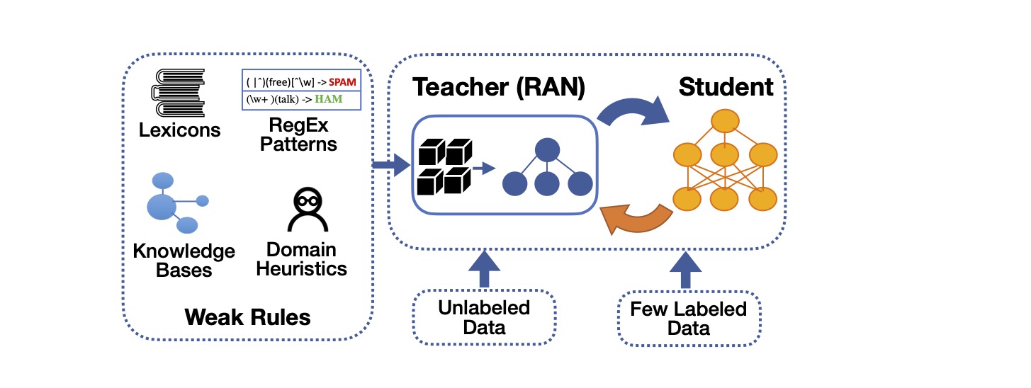
Main components:
* **Weak Rules**: domain-specific rules, expressed as Python labeling functions. Weak supervision usually considers multiple rules that rely on heuristics (e.g., regular expressions) for annotating text instances with weak labels.
* **Student**: a base model (e.g., a BERT-based classifier) that provides pseudo-labels as in standard self-training. In contrast to heuristic rules that cover a subset of the instances, the student can predict pseudo-labels for all instances.
* **RAN Teacher**: our Rule Attention Teacher Network that aggregates the predictions of multiple weak sources (rules and student) with instance-specific weights to compute a single pseudo-label for each instance.
The following table reports classification results over 6 benchmark datasets averaged over multiple runs.
Method | TREC | SMS | YouTube | CENSUS | MIT-R | Spouse
--- | --- | --- | --- |--- |--- |---
Majority Voting | 60.9 | 48.4 | 82.2 | 80.1 | 40.9 | 44.2
Snorkel | 65.3 | 94.7 | 93.5 | 79.1 | 75.6 | 49.2
Classic Self-training | 71.1 | 95.1 | 92.5 | 78.6 | 72.3 | 51.4
**ASTRA** | **80.3** | **95.3** | **95.3** | **83.1** | **76.1** | **62.3**
Our [NAACL'21 paper](https://www.microsoft.com/en-us/research/publication/leaving-no-valuable-knowledge-behind-weak-supervision-with-self-training-and-domain-specific-rules/) describes our ASTRA framework and more experimental results in detail.
## Installation
First, create a conda environment running Python 3.6:
```
conda create --name astra python=3.6
conda activate astra
```
Then, install the required dependencies:
```
pip install -r requirements.txt
```
## Download Data
For reproducibility, you can directly download our pre-processed data files (split into multiple unlabeled/train/dev sets):
```
cd data
bash prepare_data.sh
```
The original datasets are available [here](https://github.com/awasthiabhijeet/Learning-From-Rules).
## Running ASTRA
To replicate our NAACL '21 experiments, you can directly run our bash script:
```
cd scripts
bash run_experiments.sh
```
The above script will run ASTRA and report results under a new "experiments" folder.
You can alternatively run ASTRA with custom arguments as:
```
cd astra
python main.py --dataset <DATASET> --student_name <STUDENT> --teacher_name <TEACHER>
```
Supported STUDENT models:
1. **logreg**: Bag-of-words Logistic Regression classifier
2. **elmo**: ELMO-based classifier
3. **bert**: BERT-based classifier
Supported TEACHER models:
1. **ran**: our Rule Attention Network (RAN)
We will soon add instructions for supporting custom datasets as well as student and teacher components.
## Citation
```
@InProceedings{karamanolakis2021self-training,
author = {Karamanolakis, Giannis and Mukherjee, Subhabrata (Subho) and Zheng, Guoqing and Awadallah, Ahmed H.},
title = {Self-training with Weak Supervision},
booktitle = {NAACL 2021},
year = {2021},
month = {May},
publisher = {NAACL 2021},
url = {https://www.microsoft.com/en-us/research/publication/self-training-weak-supervision-astra/},
}
```
## Contributing
This project welcomes contributions and suggestions. Most contributions require you to agree to a
Contributor License Agreement (CLA) declaring that you have the right to, and actually do, grant us
the rights to use your contribution. For details, visit https://cla.opensource.microsoft.com.
When you submit a pull request, a CLA bot will automatically determine whether you need to provide
a CLA and decorate the PR appropriately (e.g., status check, comment). Simply follow the instructions
provided by the bot. You will only need to do this once across all repos using our CLA.
This project has adopted the [Microsoft Open Source Code of Conduct](https://opensource.microsoft.com/codeofconduct/).
For more information see the [Code of Conduct FAQ](https://opensource.microsoft.com/codeofconduct/faq/) or
contact [opencode@microsoft.com](mailto:opencode@microsoft.com) with any additional questions or comments.
## Trademarks
This project may contain trademarks or logos for projects, products, or services. Authorized use of Microsoft
trademarks or logos is subject to and must follow
[Microsoft's Trademark & Brand Guidelines](https://www.microsoft.com/en-us/legal/intellectualproperty/trademarks/usage/general).
Use of Microsoft trademarks or logos in modified versions of this project must not cause confusion or imply Microsoft sponsorship.
Any use of third-party trademarks or logos are subject to those third-party's policies.
| ASTRA/README.md/0 | {
"file_path": "ASTRA/README.md",
"repo_id": "ASTRA",
"token_count": 1498
} | 20 |
from .LogReg import LogRegTrainer
from .BERT import BertTrainer
from .default_model import DefaultModelTrainer | ASTRA/astra/model/__init__.py/0 | {
"file_path": "ASTRA/astra/model/__init__.py",
"repo_id": "ASTRA",
"token_count": 29
} | 21 |
. ./venv/bin/activate
sudo apt install default-jre -y
seed=110
n_experts=8
vv=lora_adamix
while [[ $# -gt 0 ]]
do
key="$1"
case $key in
--seed)
seed=$2
shift
shift
;;
--n_experts)
n_experts=$2
shift
shift
;;
--vv)
vv=$2
shift
shift
;;
esac
done
python -m torch.distributed.launch --nproc_per_node=16 src/gpt2_beam.py \
--data ./data/e2e/test.jsonl \
--batch_size 1 \
--seq_len 128 \
--eval_len 64 \
--model_card gpt2.md \
--init_checkpoint ./trained_models/GPT2_M/e2e/$seed/$vv/model.final.pt \
--platform local \
--lora_dim 4 \
--lora_alpha 32 \
--beam 10 \
--length_penalty 0.8 \
--no_repeat_ngram_size 4 \
--repetition_penalty 1.0 \
--eos_token_id 628 \
--work_dir ./trained_models/GPT2_M/e2e/$seed/$vv \
--output_file predict.jsonl \
--n_experts $n_experts \
--share_A 0 \
--share_B 1
python src/gpt2_decode.py \
--vocab ./vocab \
--sample_file ./trained_models/GPT2_M/e2e/$seed/$vv/predict.jsonl \
--input_file ./data/e2e/test_formatted.jsonl \
--output_ref_file e2e_ref.txt \
--output_pred_file e2e_pred.txt
python eval/e2e/measure_scores.py e2e_ref.txt e2e_pred.txt -p | AdaMix/NLG/run_eval_e2e.sh/0 | {
"file_path": "AdaMix/NLG/run_eval_e2e.sh",
"repo_id": "AdaMix",
"token_count": 605
} | 22 |
# ------------------------------------------------------------------------------------------
# Copyright (c). All rights reserved.
# Licensed under the MIT License (MIT). See LICENSE in the repo root for license information.
# ------------------------------------------------------------------------------------------
import sys
import io
import json
with open(sys.argv[1], 'r', encoding='utf8') as reader, \
open(sys.argv[2], 'w', encoding='utf8') as writer :
lines_dict = json.load(reader)
full_rela_lst = []
full_src_lst = []
full_tgt_lst = []
unique_src = 0
for example in lines_dict:
rela_lst = []
temp_triples = ''
for i, tripleset in enumerate(example['tripleset']):
subj, rela, obj = tripleset
rela = rela.lower()
rela_lst.append(rela)
if i > 0:
temp_triples += ' | '
temp_triples += '{} : {} : {}'.format(subj, rela, obj)
unique_src += 1
for sent in example['annotations']:
full_tgt_lst.append(sent['text'])
full_src_lst.append(temp_triples)
full_rela_lst.append(rela_lst)
print('unique source is', unique_src)
for src, tgt in zip(full_src_lst, full_tgt_lst):
x = {}
x['context'] = src # context #+ '||'
x['completion'] = tgt #completion
writer.write(json.dumps(x)+'\n') | AdaMix/NLG/src/format_converting_dart.py/0 | {
"file_path": "AdaMix/NLG/src/format_converting_dart.py",
"repo_id": "AdaMix",
"token_count": 597
} | 23 |
<!---
Copyright 2020 The HuggingFace Team. All rights reserved.
Licensed under the Apache License, Version 2.0 (the "License");
you may not use this file except in compliance with the License.
You may obtain a copy of the License at
http://www.apache.org/licenses/LICENSE-2.0
Unless required by applicable law or agreed to in writing, software
distributed under the License is distributed on an "AS IS" BASIS,
WITHOUT WARRANTIES OR CONDITIONS OF ANY KIND, either express or implied.
See the License for the specific language governing permissions and
limitations under the License.
-->
# Generating the documentation
To generate the documentation, you first have to build it. Several packages are necessary to build the doc,
you can install them with the following command, at the root of the code repository:
```bash
pip install -e ".[docs]"
```
---
**NOTE**
You only need to generate the documentation to inspect it locally (if you're planning changes and want to
check how they look like before committing for instance). You don't have to commit the built documentation.
---
## Packages installed
Here's an overview of all the packages installed. If you ran the previous command installing all packages from
`requirements.txt`, you do not need to run the following commands.
Building it requires the package `sphinx` that you can
install using:
```bash
pip install -U sphinx
```
You would also need the custom installed [theme](https://github.com/readthedocs/sphinx_rtd_theme) by
[Read The Docs](https://readthedocs.org/). You can install it using the following command:
```bash
pip install sphinx_rtd_theme
```
The third necessary package is the `recommonmark` package to accept Markdown as well as Restructured text:
```bash
pip install recommonmark
```
## Building the documentation
Once you have setup `sphinx`, you can build the documentation by running the following command in the `/docs` folder:
```bash
make html
```
A folder called ``_build/html`` should have been created. You can now open the file ``_build/html/index.html`` in your
browser.
---
**NOTE**
If you are adding/removing elements from the toc-tree or from any structural item, it is recommended to clean the build
directory before rebuilding. Run the following command to clean and build:
```bash
make clean && make html
```
---
It should build the static app that will be available under `/docs/_build/html`
## Adding a new element to the tree (toc-tree)
Accepted files are reStructuredText (.rst) and Markdown (.md). Create a file with its extension and put it
in the source directory. You can then link it to the toc-tree by putting the filename without the extension.
## Preview the documentation in a pull request
Once you have made your pull request, you can check what the documentation will look like after it's merged by
following these steps:
- Look at the checks at the bottom of the conversation page of your PR (you may need to click on "show all checks" to
expand them).
- Click on "details" next to the `ci/circleci: build_doc` check.
- In the new window, click on the "Artifacts" tab.
- Locate the file "docs/_build/html/index.html" (or any specific page you want to check) and click on it to get a
preview.
## Writing Documentation - Specification
The `huggingface/transformers` documentation follows the
[Google documentation](https://sphinxcontrib-napoleon.readthedocs.io/en/latest/example_google.html) style. It is
mostly written in ReStructuredText
([Sphinx simple documentation](https://www.sphinx-doc.org/en/master/usage/restructuredtext/index.html),
[Sourceforge complete documentation](https://docutils.sourceforge.io/docs/ref/rst/restructuredtext.html)).
### Adding a new tutorial
Adding a new tutorial or section is done in two steps:
- Add a new file under `./source`. This file can either be ReStructuredText (.rst) or Markdown (.md).
- Link that file in `./source/index.rst` on the correct toc-tree.
Make sure to put your new file under the proper section. It's unlikely to go in the first section (*Get Started*), so
depending on the intended targets (beginners, more advanced users or researchers) it should go in section two, three or
four.
### Adding a new model
When adding a new model:
- Create a file `xxx.rst` under `./source/model_doc` (don't hesitate to copy an existing file as template).
- Link that file in `./source/index.rst` on the `model_doc` toc-tree.
- Write a short overview of the model:
- Overview with paper & authors
- Paper abstract
- Tips and tricks and how to use it best
- Add the classes that should be linked in the model. This generally includes the configuration, the tokenizer, and
every model of that class (the base model, alongside models with additional heads), both in PyTorch and TensorFlow.
The order is generally:
- Configuration,
- Tokenizer
- PyTorch base model
- PyTorch head models
- TensorFlow base model
- TensorFlow head models
These classes should be added using the RST syntax. Usually as follows:
```
XXXConfig
~~~~~~~~~~~~~~~~~~~~~~~~~~~~~~~~~~~~~~~~~~~~~~~~~~~~~~~~~~~~~~~~~~~~~~~~~~~~~~~~~~~~~~~~~~~~~~~~~~~~~~~~~~~~~~~~~~~~~~~
.. autoclass:: transformers.XXXConfig
:members:
```
This will include every public method of the configuration that is documented. If for some reason you wish for a method
not to be displayed in the documentation, you can do so by specifying which methods should be in the docs:
```
XXXTokenizer
~~~~~~~~~~~~~~~~~~~~~~~~~~~~~~~~~~~~~~~~~~~~~~~~~~~~~~~~~~~~~~~~~~~~~~~~~~~~~~~~~~~~~~~~~~~~~~~~~~~~~~~~~~~~~~~~~~~~~~~
.. autoclass:: transformers.XXXTokenizer
:members: build_inputs_with_special_tokens, get_special_tokens_mask,
create_token_type_ids_from_sequences, save_vocabulary
```
### Writing source documentation
Values that should be put in `code` should either be surrounded by double backticks: \`\`like so\`\` or be written as
an object using the :obj: syntax: :obj:\`like so\`. Note that argument names and objects like True, None or any strings
should usually be put in `code`.
When mentionning a class, it is recommended to use the :class: syntax as the mentioned class will be automatically
linked by Sphinx: :class:\`~transformers.XXXClass\`
When mentioning a function, it is recommended to use the :func: syntax as the mentioned function will be automatically
linked by Sphinx: :func:\`~transformers.function\`.
When mentioning a method, it is recommended to use the :meth: syntax as the mentioned method will be automatically
linked by Sphinx: :meth:\`~transformers.XXXClass.method\`.
Links should be done as so (note the double underscore at the end): \`text for the link <./local-link-or-global-link#loc>\`__
#### Defining arguments in a method
Arguments should be defined with the `Args:` prefix, followed by a line return and an indentation.
The argument should be followed by its type, with its shape if it is a tensor, and a line return.
Another indentation is necessary before writing the description of the argument.
Here's an example showcasing everything so far:
```
Args:
input_ids (:obj:`torch.LongTensor` of shape :obj:`(batch_size, sequence_length)`):
Indices of input sequence tokens in the vocabulary.
Indices can be obtained using :class:`~transformers.AlbertTokenizer`.
See :meth:`~transformers.PreTrainedTokenizer.encode` and
:meth:`~transformers.PreTrainedTokenizer.__call__` for details.
`What are input IDs? <../glossary.html#input-ids>`__
```
For optional arguments or arguments with defaults we follow the following syntax: imagine we have a function with the
following signature:
```
def my_function(x: str = None, a: float = 1):
```
then its documentation should look like this:
```
Args:
x (:obj:`str`, `optional`):
This argument controls ...
a (:obj:`float`, `optional`, defaults to 1):
This argument is used to ...
```
Note that we always omit the "defaults to :obj:\`None\`" when None is the default for any argument. Also note that even
if the first line describing your argument type and its default gets long, you can't break it on several lines. You can
however write as many lines as you want in the indented description (see the example above with `input_ids`).
#### Writing a multi-line code block
Multi-line code blocks can be useful for displaying examples. They are done like so:
```
Example::
# first line of code
# second line
# etc
```
The `Example` string at the beginning can be replaced by anything as long as there are two semicolons following it.
We follow the [doctest](https://docs.python.org/3/library/doctest.html) syntax for the examples to automatically test
the results stay consistent with the library.
#### Writing a return block
Arguments should be defined with the `Args:` prefix, followed by a line return and an indentation.
The first line should be the type of the return, followed by a line return. No need to indent further for the elements
building the return.
Here's an example for tuple return, comprising several objects:
```
Returns:
:obj:`tuple(torch.FloatTensor)` comprising various elements depending on the configuration (:class:`~transformers.BertConfig`) and inputs:
loss (`optional`, returned when ``masked_lm_labels`` is provided) ``torch.FloatTensor`` of shape ``(1,)``:
Total loss as the sum of the masked language modeling loss and the next sequence prediction (classification) loss.
prediction_scores (:obj:`torch.FloatTensor` of shape :obj:`(batch_size, sequence_length, config.vocab_size)`)
Prediction scores of the language modeling head (scores for each vocabulary token before SoftMax).
```
Here's an example for a single value return:
```
Returns:
:obj:`List[int]`: A list of integers in the range [0, 1] --- 1 for a special token, 0 for a sequence token.
```
#### Adding a new section
In ReST section headers are designated as such with the help of a line of underlying characters, e.g.,:
```
Section 1
^^^^^^^^^^^^^^^^^^
Sub-section 1
~~~~~~~~~~~~~~~~~~
```
ReST allows the use of any characters to designate different section levels, as long as they are used consistently within the same document. For details see [sections doc](https://www.sphinx-doc.org/en/master/usage/restructuredtext/basics.html#sections). Because there is no standard different documents often end up using different characters for the same levels which makes it very difficult to know which character to use when creating a new section.
Specifically, if when running `make docs` you get an error like:
```
docs/source/main_classes/trainer.rst:127:Title level inconsistent:
```
you picked an inconsistent character for some of the levels.
But how do you know which characters you must use for an already existing level or when adding a new level?
You can use this helper script:
```
perl -ne '/^(.)\1{100,}/ && do { $h{$1}=++$c if !$h{$1} }; END { %h = reverse %h ; print "$_ $h{$_}\n" for sort keys %h}' docs/source/main_classes/trainer.rst
1 -
2 ~
3 ^
4 =
5 "
```
This tells you which characters have already been assigned for each level.
So using this particular example's output -- if your current section's header uses `=` as its underline character, you now know you're at level 4, and if you want to add a sub-section header you know you want `"` as it'd level 5.
If you needed to add yet another sub-level, then pick a character that is not used already. That is you must pick a character that is not in the output of that script.
Here is the full list of characters that can be used in this context: `= - ` : ' " ~ ^ _ * + # < >`
| AdaMix/docs/README.md/0 | {
"file_path": "AdaMix/docs/README.md",
"repo_id": "AdaMix",
"token_count": 3321
} | 24 |
End of preview. Expand
in Dataset Viewer.
README.md exists but content is empty.
Use the Edit dataset card button to edit it.
- Downloads last month
- 0