Stable Cascade

This is the official codebase for Stable Cascade. We provide training & inference scripts, as well as a variety of different models you can use.
This model is built upon the Würstchen architecture and its main
difference to other models, like Stable Diffusion, is that it is working at a much smaller latent space. Why is this
important? The smaller the latent space, the faster you can run inference and the cheaper the training becomes.
How small is the latent space? Stable Diffusion uses a compression factor of 8, resulting in a 1024x1024 image being
encoded to 128x128. Stable Cascade achieves a compression factor of 42, meaning that it is possible to encode a
1024x1024 image to 24x24, while maintaining crisp reconstructions. The text-conditional model is then trained in the
highly compressed latent space. Previous versions of this architecture, achieved a 16x cost reduction over Stable
Diffusion 1.5.
Therefore, this kind of model is well suited for usages where efficiency is important. Furthermore, all known extensions
like finetuning, LoRA, ControlNet, IP-Adapter, LCM etc. are possible with this method as well. A few of those are
already provided (finetuning, ControlNet, LoRA) in the training and inference sections.
Moreover, Stable Cascade achieves impressive results, both visually and evaluation wise. According to our evaluation,
Stable Cascade performs best in both prompt alignment and aesthetic quality in almost all comparisons. The above picture
shows the results from a human evaluation using a mix of parti-prompts (link) and aesthetic prompts. Specifically,
Stable Cascade (30 inference steps) was compared against Playground v2 (50 inference steps), SDXL (50 inference steps),
SDXL Turbo (1 inference step) and Würstchen v2 (30 inference steps).

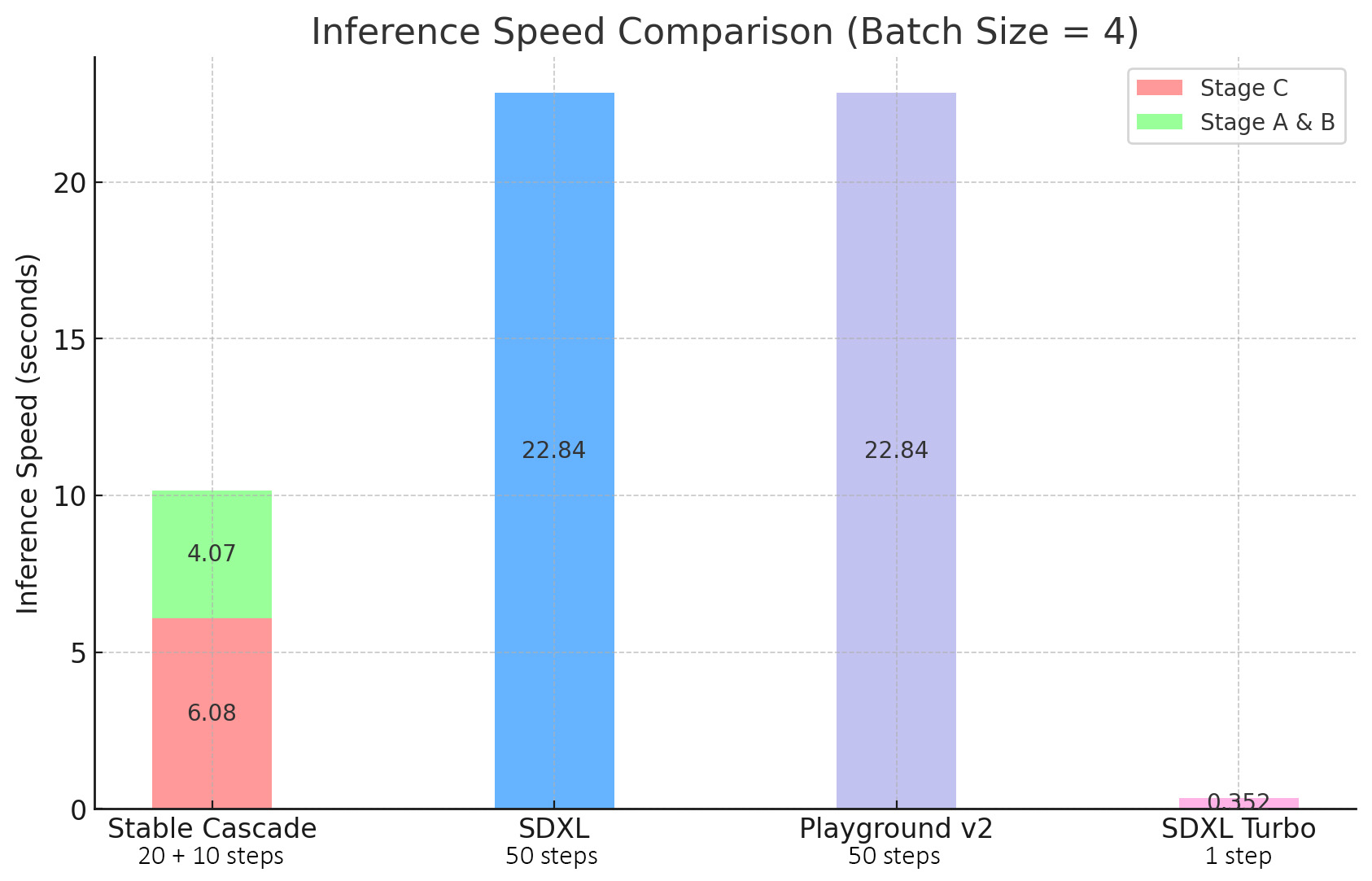
Stable Cascade´s focus on efficiency is evidenced through its architecture and a higher compressed latent space. Despite the largest model containing 1.4 billion parameters more than Stable Diffusion XL, it still features faster inference times, as can be seen in the figure below.


Model Overview
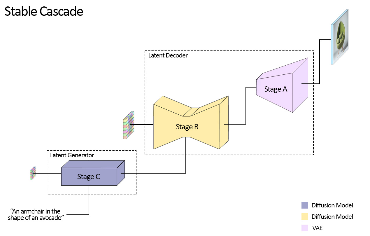
Stable Cascade consists of three models: Stage A, Stage B and Stage C, representing a cascade for generating images, hence the name "Stable Cascade". Stage A & B are used to compress images, similarly to what the job of the VAE is in Stable Diffusion. However, as mentioned before, with this setup a much higher compression of images can be achieved. Furthermore, Stage C is responsible for generating the small 24 x 24 latents given a text prompt. The following picture shows this visually. Note that Stage A is a VAE and both Stage B & C are diffusion models.

For this release, we are providing two checkpoints for Stage C, two for Stage B and one for Stage A. Stage C comes with a 1 billion and 3.6 billion parameter version, but we highly recommend using the 3.6 billion version, as most work was put into its finetuning. The two versions for Stage B amount to 700 million and 1.5 billion parameters. Both achieve great results, however the 1.5 billion excels at reconstructing small and fine details. Therefore, you will achieve the best results if you use the larger variant of each. Lastly, Stage A contains 20 million parameters and is fixed due to its small size.
Getting Started
This section will briefly outline how you can get started with Stable Cascade.
Inference
Running the model can be done through the notebooks provided in the inference section. You will find more details regarding downloading the models, compute requirements as well as some tutorials on how to use the models. Specifically, there are four notebooks provided for the following use-cases:
Text-to-Image
A compact notebook that provides you with basic functionality for text-to-image, image-variation and image-to-image.
- Text-to-Image
Cinematic photo of an anthropomorphic penguin sitting in a cafe reading a book and having a coffee.

- Image Variation
The model can also understand image embeddings, which makes it possible to generate variations of a given image (left). There was no prompt given here.

- Image-to-Image
This works just as usual, by noising an image up to a specific point and then letting the model generate from that
starting point. Here the left image is noised to 80% and the caption is: A person riding a rodent.

Furthermore, the model is also accessible in the diffusers 🤗 library. You can find the documentation and usage here.
ControlNet
This notebook shows how to use ControlNets that were trained by us or how to use one that you trained yourself for Stable Cascade. With this release, we provide the following ControlNets:
- Inpainting / Outpainting

- Face Identity

Note: The Face Identity ControlNet will be released at a later point.
- Canny

- Super Resolution

These can all be used through the same notebook and only require changing the config for each ControlNet. More information is provided in the inference guide.
LoRA
We also provide our own implementation for training and using LoRAs with Stable Cascade, which can be used to finetune the text-conditional model (Stage C). Specifically, you can add and learn new tokens and add LoRA layers to the model. This notebook shows how you can use a trained LoRA. For example, training a LoRA on my dog with the following kind of training images:

Lets me generate the following images of my dog given the prompt:
Cinematic photo of a dog [fernando] wearing a space suit.

Image Reconstruction
Lastly, one thing that might be very interesting for people, especially if you want to train your own text-conditional
model from scratch, maybe even with a completely different architecture than our Stage C, is to use the (Diffusion)
Autoencoder that Stable Cascade uses to be able to work in the highly compressed space. Just like people use Stable
Diffusion's VAE to train their own models (e.g. Dalle3), you could use Stage A & B in the same way, while
benefiting from a much higher compression, allowing you to train and run models faster.
The notebook shows how to encode and decode images and what specific benefits you get.
For example, say you have the following batch of images of dimension 4 x 3 x 1024 x 1024:

You can encode these images to a compressed size of 4 x 16 x 24 x 24, giving you a spatial compression factor of
1024 / 24 = 42.67. Afterwards you can use Stage A & B to decode the images back to 4 x 3 x 1024 x 1024, giving you
the following output:

As you can see, the reconstructions are surprisingly close, even for small details. Such reconstructions are not possible with a standard VAE etc. The notebook gives you more information and easy code to try it out.
Training
We provide code for training Stable Cascade from scratch, finetuning, ControlNet and LoRA. You can find a comprehensive explanation for how to do so in the training folder.
Remarks
The codebase is in early development. You might encounter unexpected errors or not perfectly optimized training and inference code. We apologize for that in advance. If there is interest, we will continue releasing updates to it, aiming to bring in the latest improvements and optimizations. Moreover, we would be more than happy to receive ideas, feedback or even updates from people that would like to contribute. Cheers.
Gradio App
First install gradio and diffusers by running:
pip3 install gradio
pip3 install accelerate # optionally
pip3 install git+https://github.com/kashif/diffusers.git@wuerstchen-v3
Then from the root of the project run this command:
PYTHONPATH=./ python3 gradio_app/app.py
Citation
@misc{pernias2023wuerstchen,
      title={Wuerstchen: An Efficient Architecture for Large-Scale Text-to-Image Diffusion Models},
      author={Pablo Pernias and Dominic Rampas and Mats L. Richter and Christopher J. Pal and Marc Aubreville},
      year={2023},
      eprint={2306.00637},
      archivePrefix={arXiv},
      primaryClass={cs.CV}
}
LICENSE
All the code from this repo is under an MIT LICENSE
The model weights, that you can get from Hugginface following these instructions, are under a STABILITY AI NON-COMMERCIAL RESEARCH COMMUNITY LICENSE